
Accuracy and Precision of Fodar Data
This blog consolidates a number of studies that have been done to assess fodar accuracy and precision, as well as reviews some related terminology and concepts that I think are important. I’ll keep updating this post over time, so check back to see the most recent updates (last updated 26 Feb 18).
The short answer is that in nearly every assessment of accuracy and precision of the maps I create, we find that accuracy is about 0-40 cm and precision is 5-25 cm at 95% the RMSE level, depending on circumstance, covering areas as small as a football field to as large as the entire west coast of Alaska, at resolutions of 3 cm or higher. These results are all the more amazing because they utilized no ground control — only data collected from my airplane were needed. Note that these specs rival or exceed the best airborne lidar, especially considering fodar point density is often 100x higher.
What is fodar?
Over four years ago now, I chose to call my methods fodar because I felt the differences with other methods were both quantitatively and qualitatively different enough to merit some verbal distinction, if only to facilitate discussion. I wanted a word that captured exactly what it is that I do — I make survey-grade topographic maps and perfectly co-registered orthophotos from the air using a cheap camera. Technically this is photogrammetry, but besides being a mouthful to say, the official definition of ‘photogrammetry’ is so impossibly broad that it is almost meaningless for discussing my application. ‘Stereo-photogrammetry” comes closer in meaning, but even more of a mouthful and it’s official definition is not specific to topographic measurements and is also overprescriptive of the method. Also since the advent of airborne lidar, traditional airborne stereo-photogrammetry for the purpose of measuring topography has largely fallen out of fashion anyway, largely because it is difficult and labor intensive to achieve the same topographic accuracy as lidar, because lidar has better ability to measure topography beneath a tree canopy, and because high-end photogrammetry hardware costs about the same as a lidar. Plus, and many may disagree with this, lidar takes much less skill to use, as evidenced by the fact that these days lidar operators and processors are entry level jobs whereas skill in traditional photogrammetry takes years to decades to develop. What we have now is a photogrammetric technique that can easily measure topography at lidar accuracy using an inexpensive camera. So the word I wanted didn’t really exist and because words like lidar and insar were closely related, I chose fodar as a portmanteau of fotos and radar (in the same way that lidar is a portmanteau of laser and radar, not an acronym) and its alliteration with lidar and insar and radar when spoken of in the same breath; I chose ‘fotos’ rather than ‘photos’ for its matching letter structure to lidar and radar as well as to avoid it becoming improperly used as acronym for ‘photo detection and ranging’ which makes little sense, though it seems to be also gaining traction anyway. And words matter, everyone into marketing knows this: using “airborne stereo-photogrammetry” is fighting an uphill battle against lidar, insar, and radar in every instance it is used. The other competing meme for stereo-photogrammetry is “SfM”, which is kind of like calling lidar “GPS”, as it just highlights a specific component of the process, and a worse component that is hidden in the black box of commercial software which we really have no idea how (or even if) it is actually implemented. So if I had to come up with a definition for fodar, it would be something like “any photogrammetric process for quantitatively measuring both the color and elevation of the earth’s surface from the air using a small-format camera”. It’s tempting to add something about SfM or specific algorithms or hardware or ground control constraints, but this may change over time and we cant keep coming up with new words each time. Or it could be broadened to include ground-based or satellite measurements, but I dont see the point, let those guys come up with their own names so that it is always clear where the measurements were made, as this matters for almost all purposes. I added ‘small-format’ cameras because these have unique challenges compares to medium and large format cameras when it comes to verifying accuracy and precision, and also because it implies these cameras are not the expensive so-called metric cameras (though all digital cameras are inherently metric) costings hundreds of thousands of dollars. I’m also tempted to add something about accuracy in the definition, since my methods are more accurate than what most drones are capable of so there is a marketing benefit to me, but in a broad sense I think it’s fine that there is a range of accuracies because there is a corresponding range of needs for accuracy — at least provided we have a standard that allows for this, such as saying “fodar at the ASPRS 10 cm accuracy class”, as this is much more meaningful than saying “survey-grade SfM photogrammetry”, as even I currently do, but the current ASPRS guidance really isn’t suited to photogrammetry using small-format cameras and even says so in the document. So overall, if we get too specific or too general, the name becomes useless, and that’s how I’ve settled on this definition, though I’m happy for feedback. My thoughts on this have evolved since I first coined the term fodar in 2013 after several years of refining and testing the technique, and you can learn more on this evolution in this paper and this paper and in my earliest blogs on fodar.
What makes my flavor of fodar so awesome?
I think it comes down to accuracy and cost — my data are just as accurate (if not more so) than any other method, yet the cost of the hardware, the ease of use in flight, the lack of need for expensive ground control, and tremendous reduction in processing labor result in much lower costs in overall production, by a factor of 10 or more from what I have seen. I describe accuracy and precision below, so for now I’ll just describe the importance of the other factors. My airborne hardware package is primarily a prosumer DSLR camera, a survey-grade GPS, and some custom electronics to make them communicate. In the air I use no laptop, no IMU, and no fancy flight director and the whole system fits nicely within much smaller planes than are typical for lidar, and can even be attached to small helicopters. I simply preplan my lines, upload them to the aviation GPS that is already there, and use it alone for navigation. The system is simple enough that I can fly without a separate equipment operator, which not only reduces cost but as importantly improves my response time — even with the best of inter-personal dynamics, adding a second person increases inertia and when dealing with short weather windows or with distant or rush projects, this inertia can have a huge ripple effect in terms of performance. That a single person operation with airborne hardware you can buy on Amazon or Ebay can create maps accurate enough to meet the most stringest USGS mapping specs without use of any ground control turns this tool into a magic wand — essentially with only a few hours planning or warning, I can fly anywhere I like, wave this magic wand, and deliver the data before a typical lidar or drone survey has deployed and surveyed their ground control. The fact that no ground control or IMU is required results primarily from accurate location of the photo-centers; imagine each photo is dangling from a string from the fixed photo centers — you must solve for the length of the strings and their tilt from nadir (as well as lens distortions, etc), but with 1000s of tie points between photos, the solution space is quite limited and actually outperforms what IMUs, ground control, and even the air control can provide. So this is not just direct georeferencing: the air control effectively seeds the bundle adjustment so that the solution falls into the right error potential well, and after that the solution of these billions of equations to solve the 15 or so unknowns (including improvement of the seeded X, Y, Z) is so ridiculously over-constrained that it outperforms our ability to pre-determine the interior or exterior orientations. From my perspective, even though the unknowns and equations to solve them are identical to traditional photogrammetry, today’s software and hardware is really doing something unique and special that simply is not feasible (or perhaps possible) to do manually. So in one sense, it’s just a new flavor of photogrammety, but I think those that see the subtleties in the bigger picture would agree that this is something new and closer to waving a magic wand over the landscape than simply being a new flavor of stereo-photogrammetry: it really is a game changer in the field of airborne remote sensing — it wont replace lidar or insar, but it is a powerful new tool in the airborne toolbag that is more appropriate to use in many circumstances currently served by those technologies. A really simple example of this is the creation of orthophotos simultaneously with lidar: as I understand it, the current state of the art is to use traditional AT involving ground control and rectifying the photos against the lidar DEM, but to me this is like bringing a knife to a gun fight. Those same photos could be processed independently to create an independent DEM at much higher resolution than the lidar which will result in a much better orthorectification, and this fodar DEM can then be fused with the lidar DEM to achieve a much denser first surface and probably used in a variety of ways algorithmically to produce a better bald-earth model more easily and inexpensively. It might even be possible to use the tilts calculated by the bundle adjustment to improve the direct georeferencing of the lidar. But I digress…
What are the strongest controls on fodar accuracy and precision?
Steep terrain tends to improve accuracy as it narrows the solution space of the bundle adjustment due to the scale variations. Single-day acquisitions tend to result in the best precision because multi-day acquisitions result in blending multiple airborne GPS solutions which can insert a bias between the photo-centers measured on different days. So, exclusive of a variety of more expensive tricks I have not shared here (that is, in my ‘budget fodar’…), in rough numbers you can expect 0-20 cm accuracy in the mountains and 10-40 cm accuracy in the flats, and 5-15 cm precision in areas less than 1000 km2 (roughly a single day maximum) and 10-25 cm precision in larger areas, all at the 95% level; the range of variability seen here using these techniques largely comes down to luck but also due to the vagaries of substandard validation techniques as described — the best methods show the tighter tolerances. The bulk of the highest error is spatially correlated, meaning that it results from small blocks of photos being offset vertically by these amounts; the random noise in the point cloud appears to remain in the 3 cm range. Larger pixels also tend to have worse precision, but this is due to spatial aliasing common to all rasterized data rather than something specific to fodar. The result for change-detection purposes is that you should generally expect spatially-correlated noise centered at the single-map precision level but extending up into double the range of precision (eg., when +20 cm meets -20 cm you get 40 cm of noise), such that you can easily measure decimeter signals without issue, as well as signals in the single centimeter range provided they occur over larger areas. All that being said, I am not tying the word ‘fodar’ to a particular accuracy spec, I believe the right way to discuss this is along the lines of the ASPRS 2014 standards which make a good first attempt to divorce technology from specifications; that is, my most economical product is fodar at the 10 to 20 cm accuracy class, provided I have at least a few GCPs to make the final affine shifts, or 20-40 cm accuracy class without GCPs.
Why is repeatability the best way to measure fodar accuracy and precision?
Along the lines of fodar being something new, here I make the case that repeat mapping is the best form of validation of fodar accuracy and precision possible, both in terms of the efficacy of that validation and its cost. In this context of my own work in measuring landscape change, what I value most is repeatability — when I map the same area twice, do I get the same answer? This approach is fundamentally different than accepted practices, which dictate that only ground control in the form of GPS should be used for validation (eg, ASPRS 2014). That specification exists because as expensive as ground control is, repeating a lidar acquisition is even more expensive and also because lidar itself often requires substantial ground control such that two acquisitions are not truly independent if they utilize that same ground control. That’s just not the case with fodar — fodar hardware is so cheap that it is much less expensive to fly all or part of an acquisition twice than acquire massive ground control and each flight is truly independent of the other (though you could nitpick and say GPS satellite geometries repeat themselves, but we are beyond the weeds at that point…). Note here that error measured in this way does not emerge from the damn lies of sampling statistics– that is, taking a hundred ground control points and claiming that you have 95% confidence that these 100 comparisons represent 100 billion other unmeasured pixels. Rather, when you compare two DEMs in this way you are validating every single pixel and saying that 95% of those measurements fall within your calculated error range — no guess work, no extrapolations, just good old-fashioned measurements. There is simply no better way to assess accuracy and precision than this, and of course the real beauty of repeat mapping as validation is that you end up with two maps and thus capture any changes that may have occurred in that interval (changes which are noise for the purposes of validation but signal for the purposes that paid for the maps in the first place). And it also allows us to not only be truly sensor agnostic but sensor component agnostic — who cares HOW your system works if every single one of your pixels on the two maps are within 10 cm of each other? Or within X meters of each other for that matter, as it’s all about meeting a spec for X.
Does repeatability measure accuracy or precision?
Before getting lost in the weeds, first consider that nearly all validation studies of my fodar maps have found that 95% of the elevations points are with 6 to 20 cm, depending on project — so consider that the answer of which type of noise that is doesn’t matter if the accuracy class of the project was 20 cm. In fact, the repeatability is a combination of accuracy and precision, and they can be disentangled further if needed. If we compare two fodar DEMs and find a mean difference of 30 cm and a standard deviation of 5 cm, then for practical purposes we can consider 30 cm the accuracy and 10 cm (roughly double the standard deviation) the precision of the fodar data. (Be aware that these values can be reported either as a standard deviation or a 95% RMSE, which is bit less than double the standard deviation. So when comparing technologies or their specifications, be sure you are comparing apples to apples. The best marketing tool is to report standard deviation because it is a smaller number, but the scientific and statistical standard is to report as 95%.) At first glance, it may seem a stretch to call this 30 cm the accuracy, but consider that each of the thousands of photo centers are pinned to within 5 cm using GPS — this is an extremely powerful form of air control which does not allow the overall solution to drift, much like the way a crystal lattice stops defects from growing. And also consider that it actually works: I’ve mapped some locations a dozen times and the solution is always within about 30 cm and I’ve compared them to ground control points and find the same — there is simply no way this could be random chance. So in this example (which is typical), all we need to do is shift one data set relative to another by 30 cm to reduce the misfit to 0 cm mean, and what we are left with is precision at the 10 cm level for 95% of measurements. The major caveat here is that if a potential 30 cm geospatial error (accuracy) matters to you, then you can’t get away from needing some ground control points that are much more accurate than 30 cm: given a fodar precision of 10 cm, a single 2 cm accuracy GCP will get your fodar accurate to at least 10 cm, and a dozen such GCPs will get you close to 2 cm. The futility of striving for 2 cm accuracy in maps considering that neither Alaska’s surface nor its tectonic plates are stable at the 2 cm level is a digression for another time…
So the point for me is that precision is everything — your accuracy could be 100s of meters off and a single ground control point can reduce that to nearly zero, but nothing will fix poor precision once the map is made (you can’t fix stupid…). So my standard method to assessing data quality is to make two maps and subtract them and then ask whether the magnitude of this difference matters and whether it is worth the cost to improve it? If the signals I am looking for are on the order of meters, then it does not matter, and collecting tons of ground control is simply throwing money away and I believe that no standards should specify such a waste of money. If I’m looking for changes on the centimeter level as measured by some other technique, then improving accuracy does matter. In this case, I would shift one of the maps to reduce the misfit to zero mean, then the misfit I am left with will be lower and technically all precision, and then I can shift them both to match whatever control is available to reduce my accuracy to the precision level or better. At this point, any future acquisitions here can just use those fodar data for ground control using the repeatability methods I described.
Note that the case for inexpensive drones is similar, but the errors are much larger when no ground control is used in the bundle adjustment that makes the DEM. Here you should expect an accuracy and precision on the order of meters, with precision usually worse than accuracy, meaning that all bets are off on the value of reducing the data to zero mean or using a single ground control point to improve the accuracy. Though both can be reduced to decimeters if substantial ground control is used in the bundle adjustment, here again my whole argument about saving money falls apart — one way or another, you need gobs of ground control for drones which are not equipped with survey-grade GPS receivers so, while repeatibility tests are still useful, they aren’t going to cut costs much. However, given that any kid with $2000 in his pocket can buy a drone and hang up a shingle saying “The Photogrammetrist is In”, I would even more strongly recommend repeat mapping as the absolute verification of accuracy and precision. That is, divorcing technology from specs means the specs must treat the technology as a black box, and in the case of drone methodology that box let’s out no light, so repeatibility is really the only way to assess what’s going on in between the ground control used. Or to put another way, given that no drone project will ever have enough ground control to pin each and every drone photo (or lidar shot or my fodar photo for that matter), you really have every reason to believe that the data are worthless outside of where you have actually checked when taking the truly sensor agnostic view of validation. That is, in my opinion of this view, all the data should be considered guilty until proven innocent.
What about horizontal accuracy?
Thus far I have been discussing vertical accuracy of the DEM, but the case is the same for horizontal accuracy — I make the claim that comparison of two fodar datasets to each other is a far superior means of assessing accuracy and precision than is comparison to “photo-identifiable” ground control, for the same cost reasons but also because the errors in the validation technique itself rival the errors they are validating. When I use this method, I typically find the two datasets are within a pixel or two. Similar to above, projects acquired on a single day typically have a better horizontal accuracy (by comparison to each other or to ground control), on the order of a pixel, though I would argue without proof that it is likely that the accuracy is on the order of 10 – 20 cm for any size pixels because this horizontal accuracy is tied to the air control control accuracy, I just rarely collect data larger than 25 cm, so I haven’t tested that out. When acquisitions span multiple days, the horizontal accuracy degrades to within 2-3 pixels, often better. Besides the advantages of comparing billions of pixels to billions of pixels by eye, computational photo-matching can be employed to determine sub-pixel accuracy. Compare this method to traditional ground control surveys — at the very best, your eye can only determine the location of the ground control on the image to within 1/2 a pixel, and if we are being honest it’s more like an entire pixel. So that means your validation technique itself has an error about as large as the error its trying to measure! All that being said, if a 30 cm geospatial accuracy matters to your project, then you can’t get around needing some ground control, at least the first time, and a few points are really useful for blunder checking as well. That is, once you have a fodar orthomosaic sucked into perfect alignment with some ground control, you can just use that ortho in the future in the way I just described. To add icing to the cake, because fodar does not use any ground control to create the maps, you can collect the control after the project is delivered and use photo-identifiable points found in the ortho. Working backwards like this is far superior to trying to transfer ground targets to the ortho, because in the ortho you have billions of pixels to chose from so that you can find points that minimize the picking error (eg, the intersection of two cracks on a road surface that you can pick by eye at the subpixel level).
Where can you find a concise list of relevant published studies?
If you want a good but informal overview of some of the ways I go about determining accuracy and precision, you could read this blog about my November 2017 trip to Botswana where I was assisting studies of elephant habitat through repeat mapping.
Here is a concise list of papers or reports that you can find online, some of which are described below in greater detail:
There are several more papers either submitted or in press as of early 2018, so check back here for updates.
You can find a lot of my data here at the State site. Turn off all of the lidar, insar, and other and most of what’s left under the SfM tab (I don’t get to choose the labels…) is mine; you can cross-reference against my blogs. Some of those data date back to 2011, long before anyone in the survey or lidar community had even heard of SfM…
What can measuring snow depth tell us about fodar accuracy and precision?
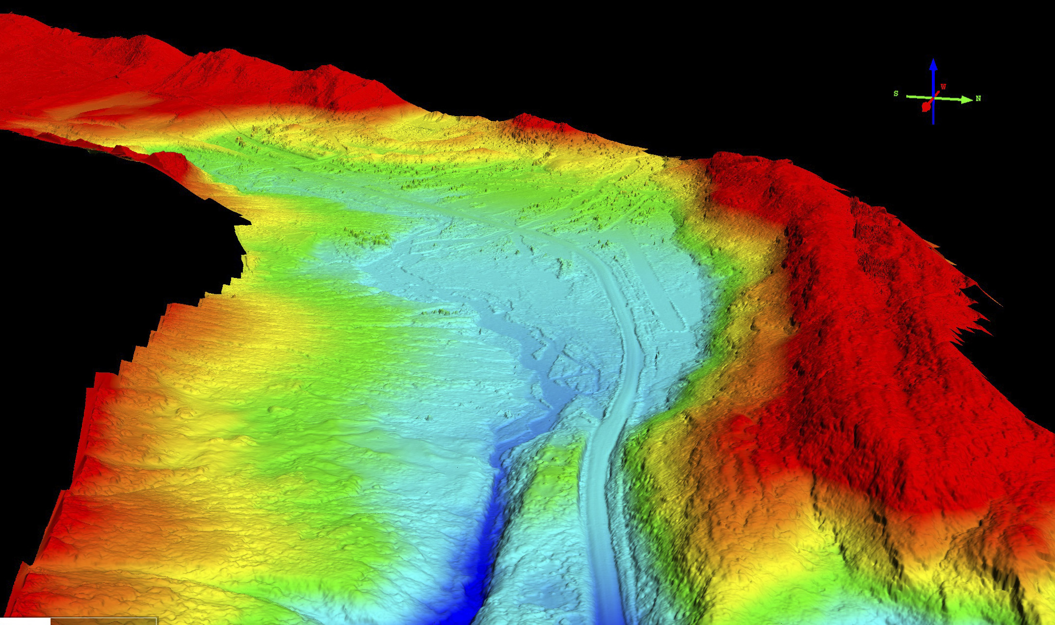
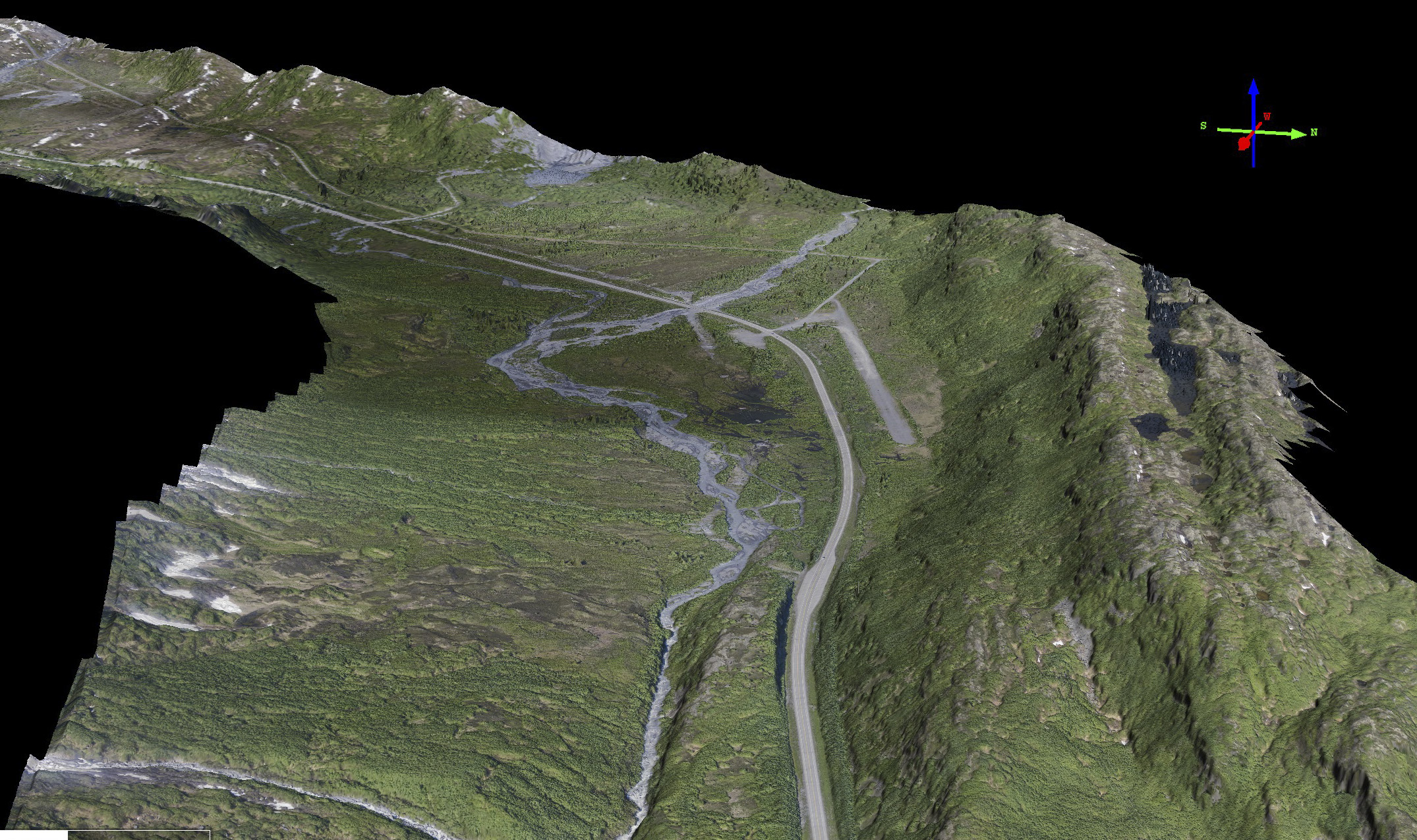
Our first formal treatment of accuracy and precision of my fodar data was made in this paper that focused on snow depths, as measured by subtracting summer topography from winter topography in arctic and sub-arctic Alaska — that is, using repeat mapping for both change detection (snow depth) and for validation of accuracy and precision. In this paper we found fodar accuracy was 30 cm and precision about 8 cm through comparison of repeat maps using my fodar system, comparison to maps made by another fodar system, and comparison to airborne lidar. We then also measured the accuracy of these difference DEMs by comparison to thousands of snow depth measurements to demonstrate that we could successfully measure snow depth (and by inference nearly any change in topography) on the centimeter level; this demonstrated that most of our errors are not spatially-correlated, such the the accuracy of the difference DEMs were about the same as the individual DEMs. I do not believe there is any other technique that can measure snow depth so well, but that’s really besides the main point. The main point is that we did measure it so well — requiring precision on the single centimeter level — which was achieved with no ground control using a $3000 camera and a GPS bought on ebay for $1200.
[pdfviewer width=”800px” height=”849px” beta=”false”]https://fairbanksfodar.com/wp-content/uploads/2015/08/nolan_etal_final_tc-9-1445-2015.pdf[/pdfviewer]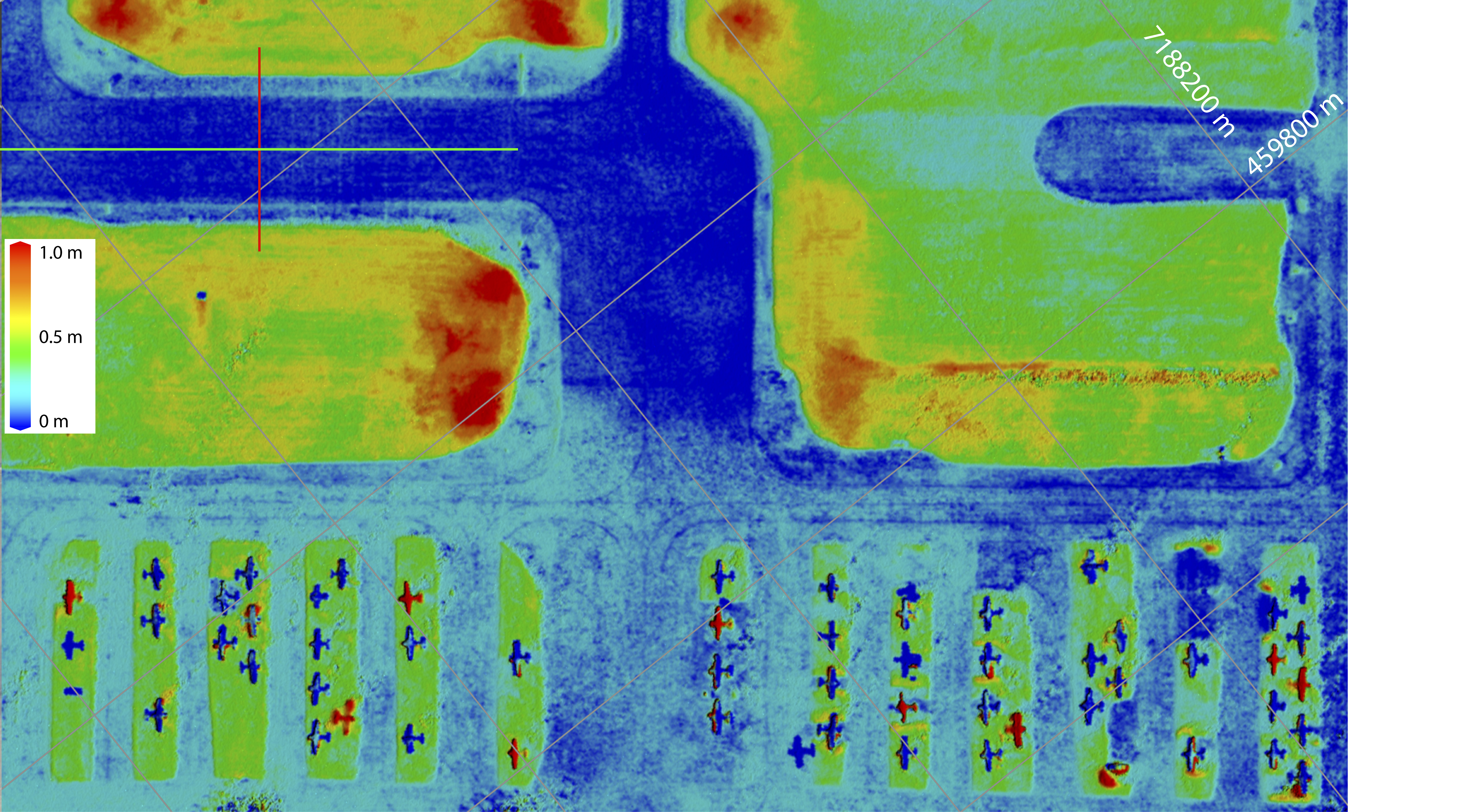
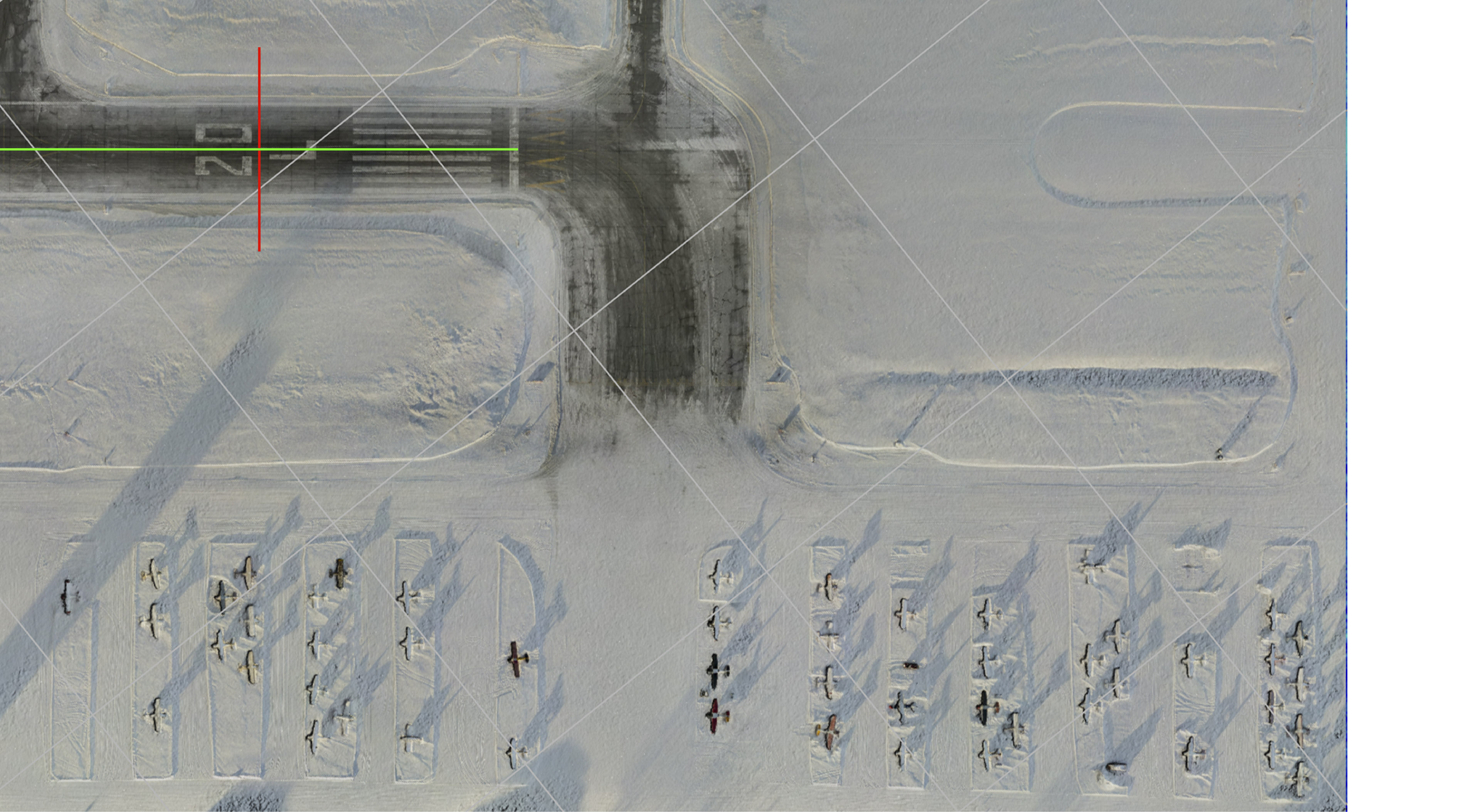
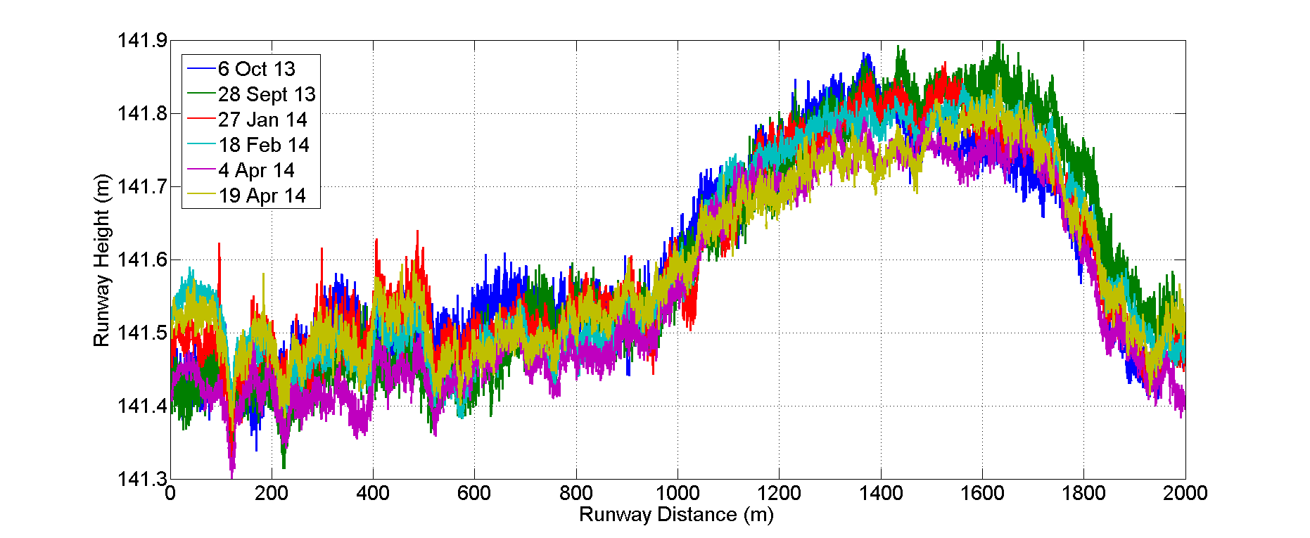
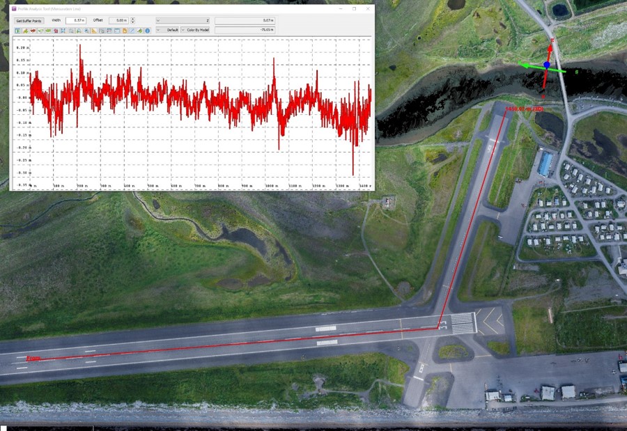
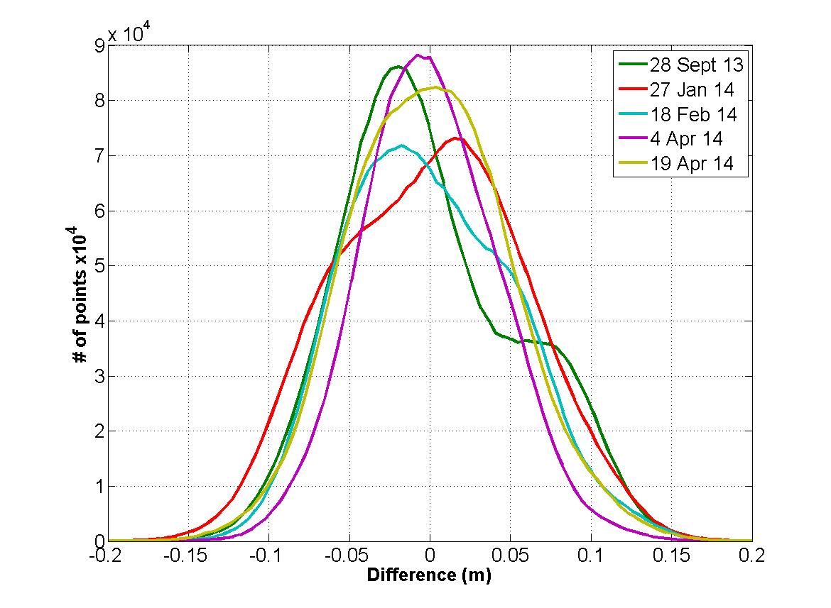
Here are elevations from six independent acquisitions down the 1+ mile length of the runway (green transect in image pair above). Note that nearly 100% of the points are within +/- 10 cm of each other, and note also that some of these differences are real, as described in the paper. This level of precision is simply remarkable, and I do not believe you will find any airborne method that can map runways better than this at any price.
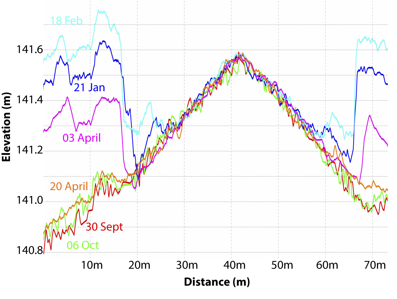
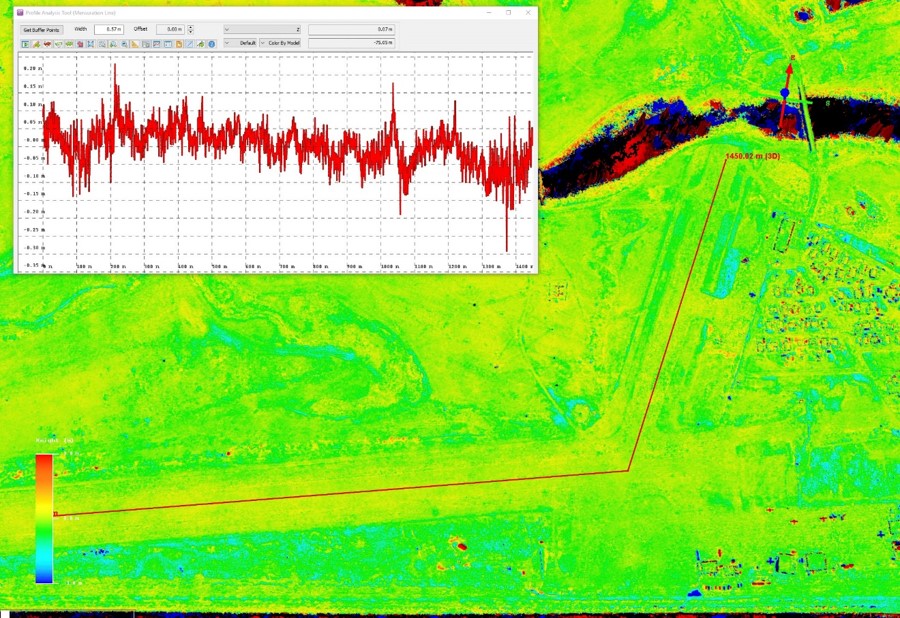
Here is a cross-profile of elevations from the runway (red line in image pair above). Not only are all of the maps capturing the runway crown, but they do so within about +/- 3 cm of each other; again, I do not believe there is an airborne technology that is superior to this, especially when you consider the price and the perfectly co-registered orthoimage that comes with it. This level of precision allows us to easily resolve the depth of snow berms surrounding the runway, which are actively plowed and change in shape throughout winter.
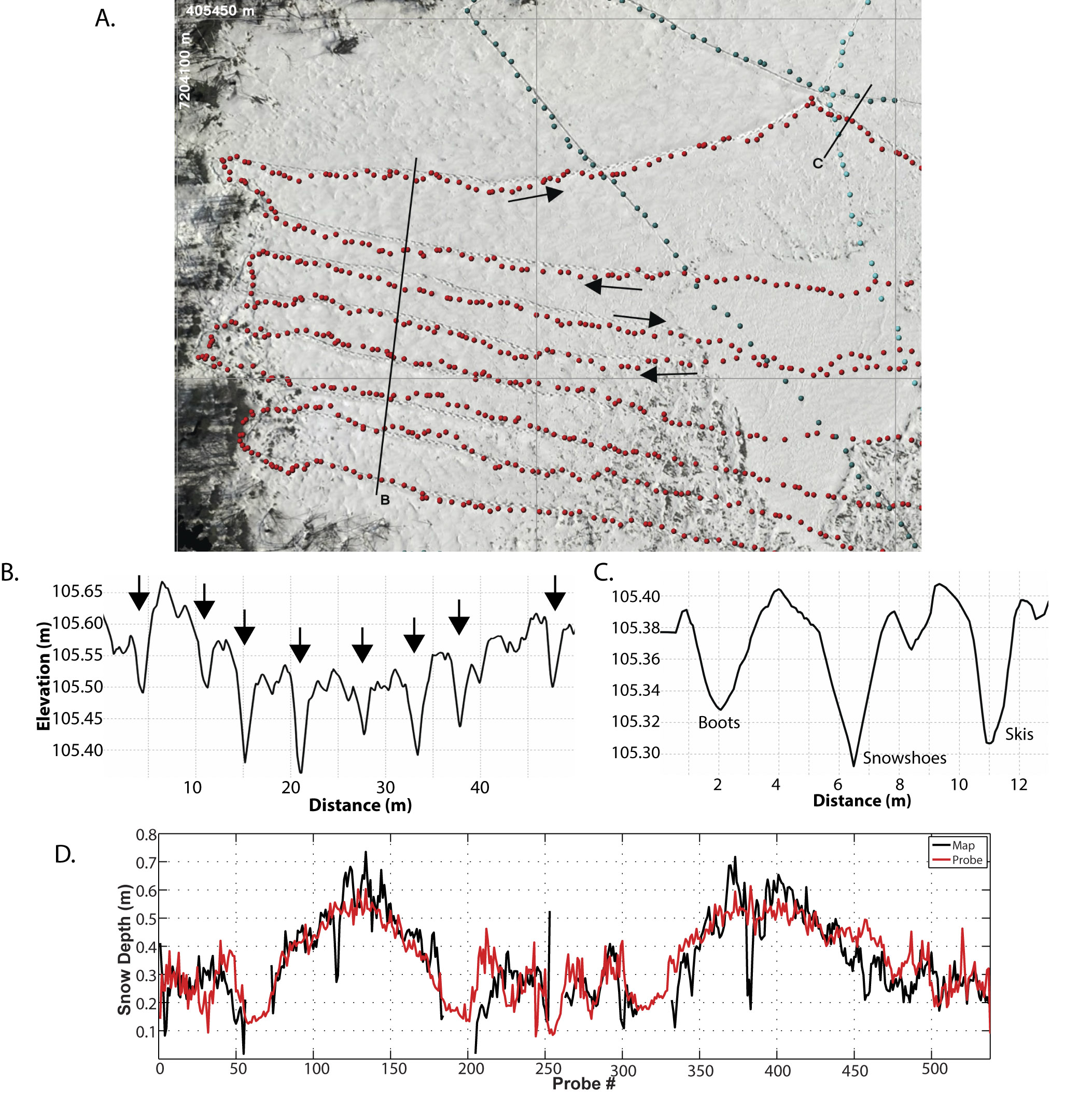
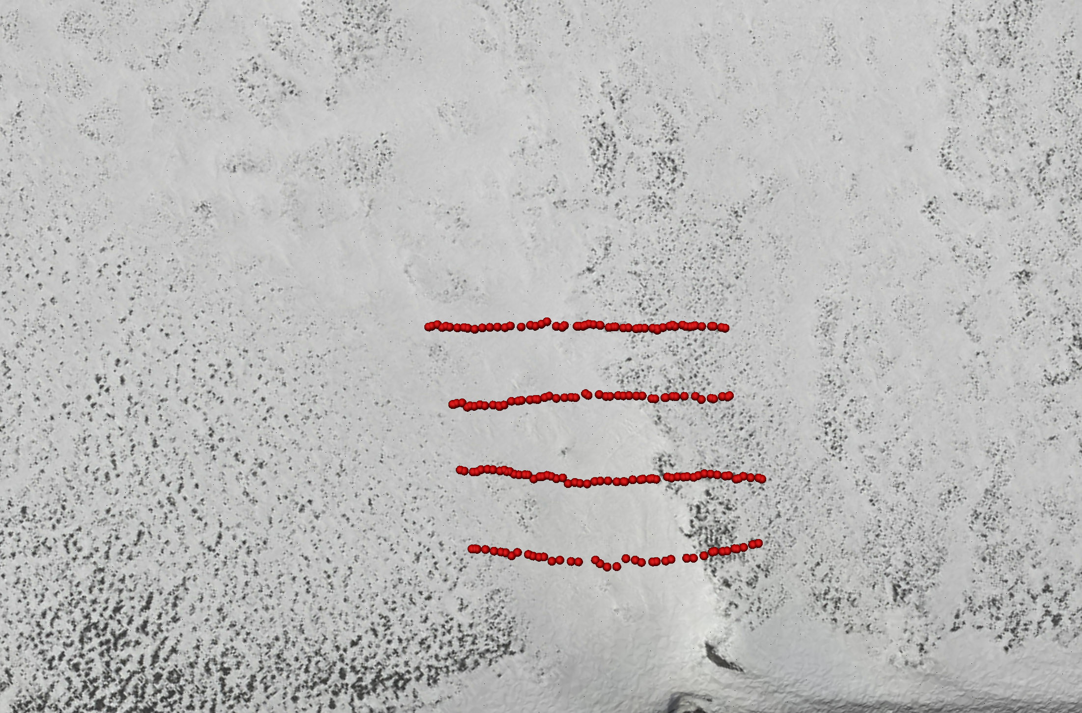
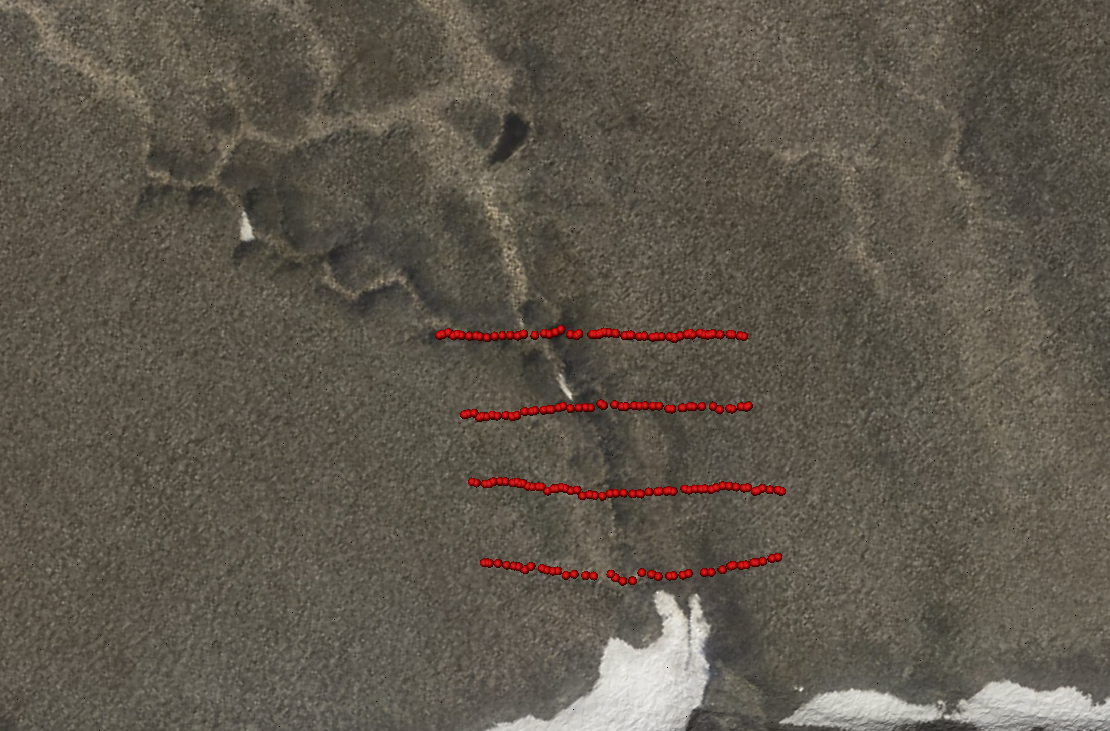
As part of this accuracy and precision assessment, we made over 6000 measurements of snow depth in the field using probes (shown as colored dots above, as measured by three people wearing different footwear). These field measurements were made before the fodar measurements, thus the footprints show up in the image and the data (arrows in B and by footwear type in C). Nevertheless, the comparison between the winter minus summer difference DEM and the probe data (D) are outstanding, and as we show in the paper are statistically identical. The major excursions are due to shrubbery being compressed in winter.
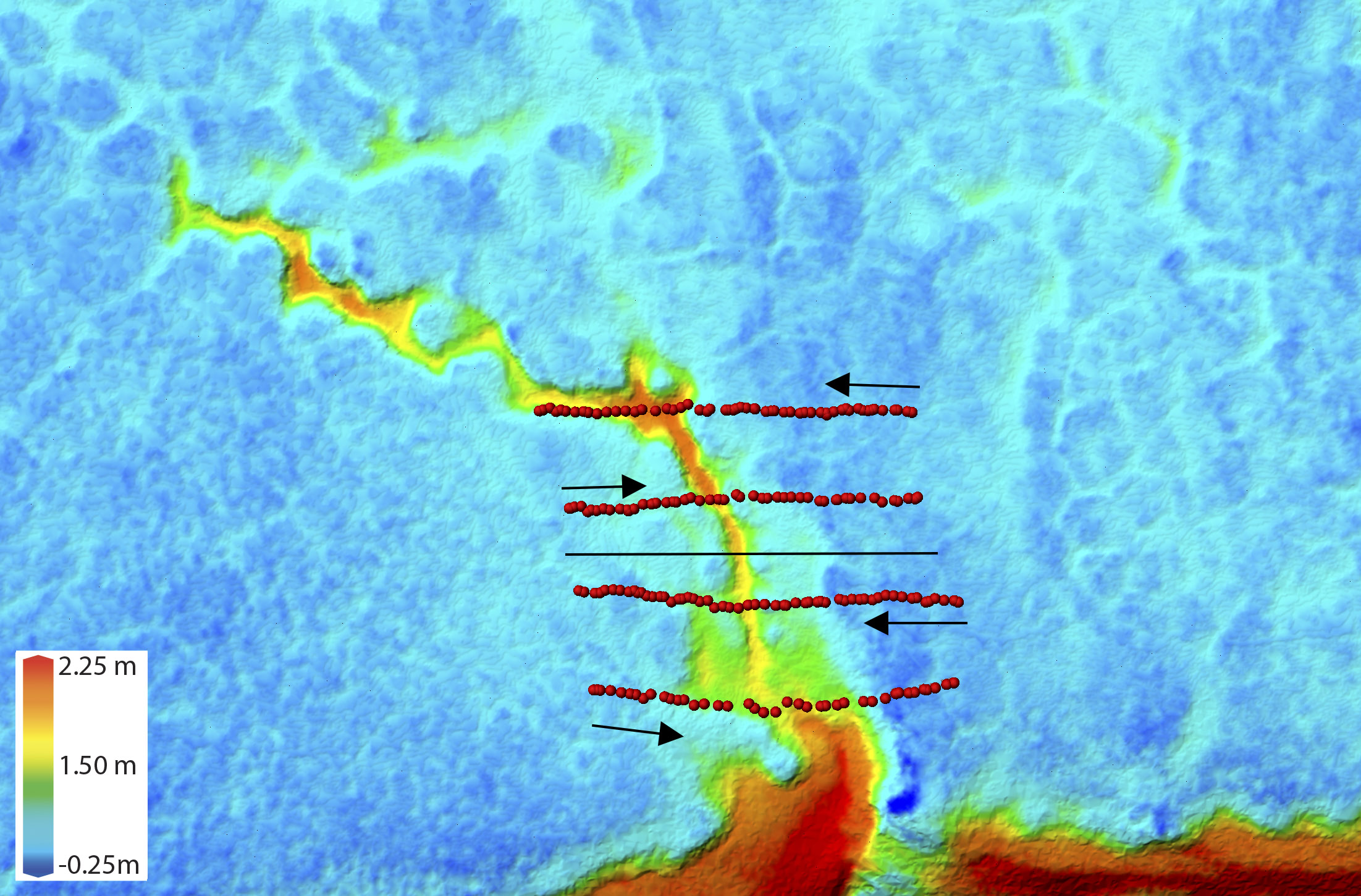
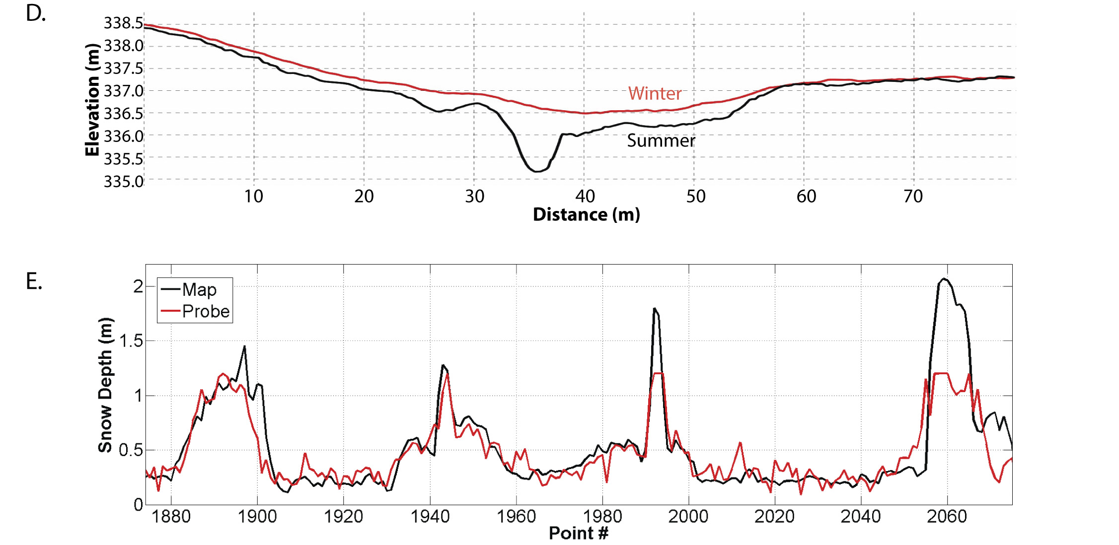
In D above, you can see the difference between the summer and winter DEM measurements seen in the previous image comparison; the distance between these lines is snow depth. In E is shown the field probe measurements compared to the fodar measurements of snow depth, back-and-forth over the gully seen in the image pairs above, with each of the four peaks in snow depth indicating where the gully was crossed. The measurements are statistically identical, with most deviations within 10 cm. The excursions above 1.3 meters are due to the snow probe being too short to reach the bottom of the gully. Our literature review in 2015 found no other published reports of measurements of snow depth with this accuracy, resolution, and spatial scale by any method, including ground methods.
What can measuring mountain peaks tell us about fodar accuracy and precision?
Our next goal after the snow paper was to confirm that we could achieve the same awesome results on steep terrain, so we decided to map the tallest peaks in the US Arctic to settle some debates on which was the tallest. To do this, I mapped the five tallest peaks 2-4 times each and we scrambled up to the top of two of them to measure with GPS. The results of the repeatability tests and the GPS comparison showed that fodar here has a vertical and horizontal accuracy of about 10 cm and a precision of about 20 cm at 95%, and that these results were superior to commercially-acquired lidar we contracted for this same study area.
[pdfviewer width=”800px” height=”849px” beta=”false”]https://fairbanksfodar.com/wp-content/uploads/2016/06/tc-10-1245-2016.pdf[/pdfviewer]This was a fun paper to work on. I developed fodar specifically to study the glaciers surrounding these peaks, so I had a lot of peak measurements in hand already. Given the mysteries of the USGS map elevations of these peaks, it was irresistible to combine my accuracy studies of glaciers and steep mountain topography with resolving that mystery.
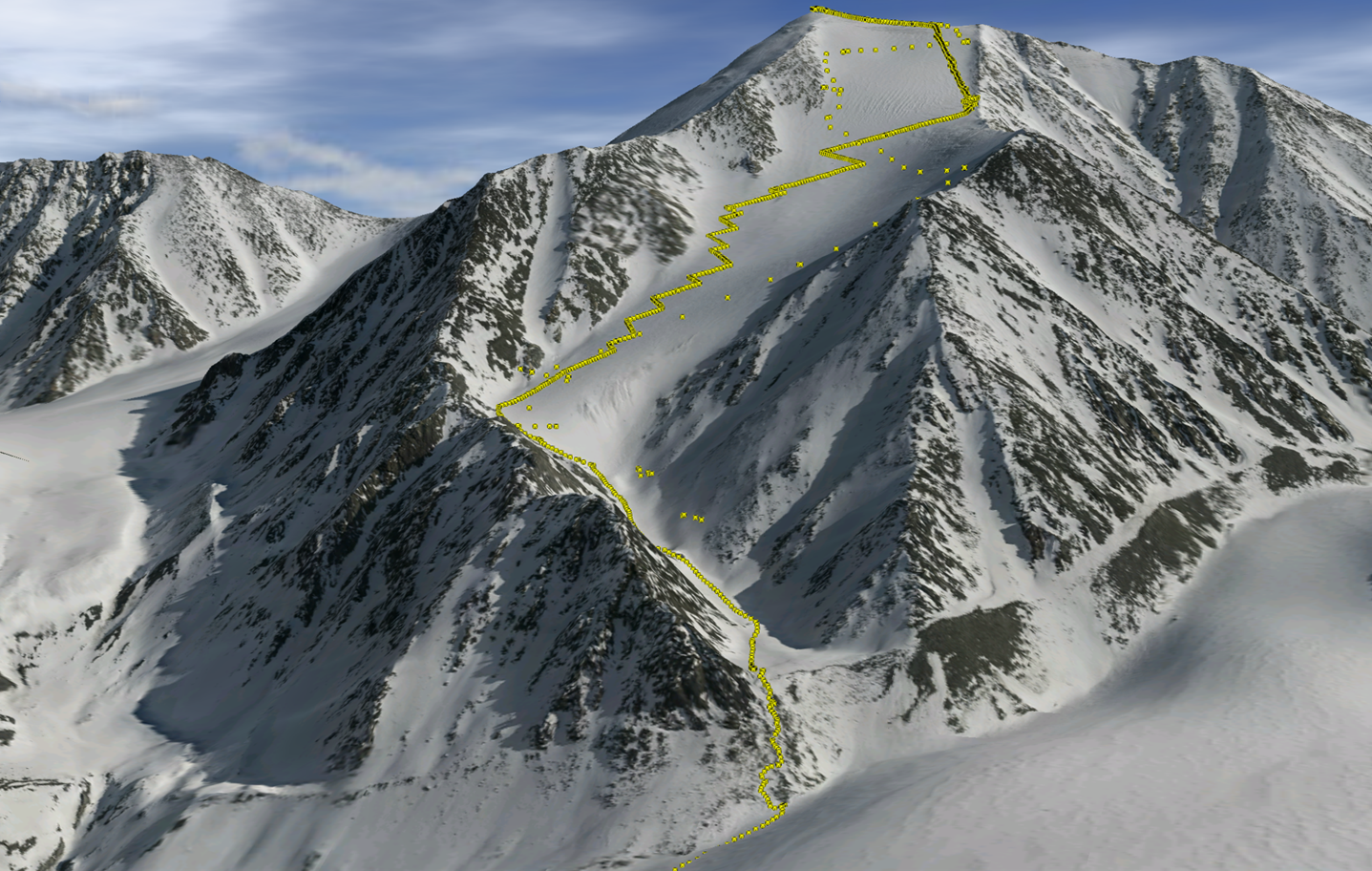
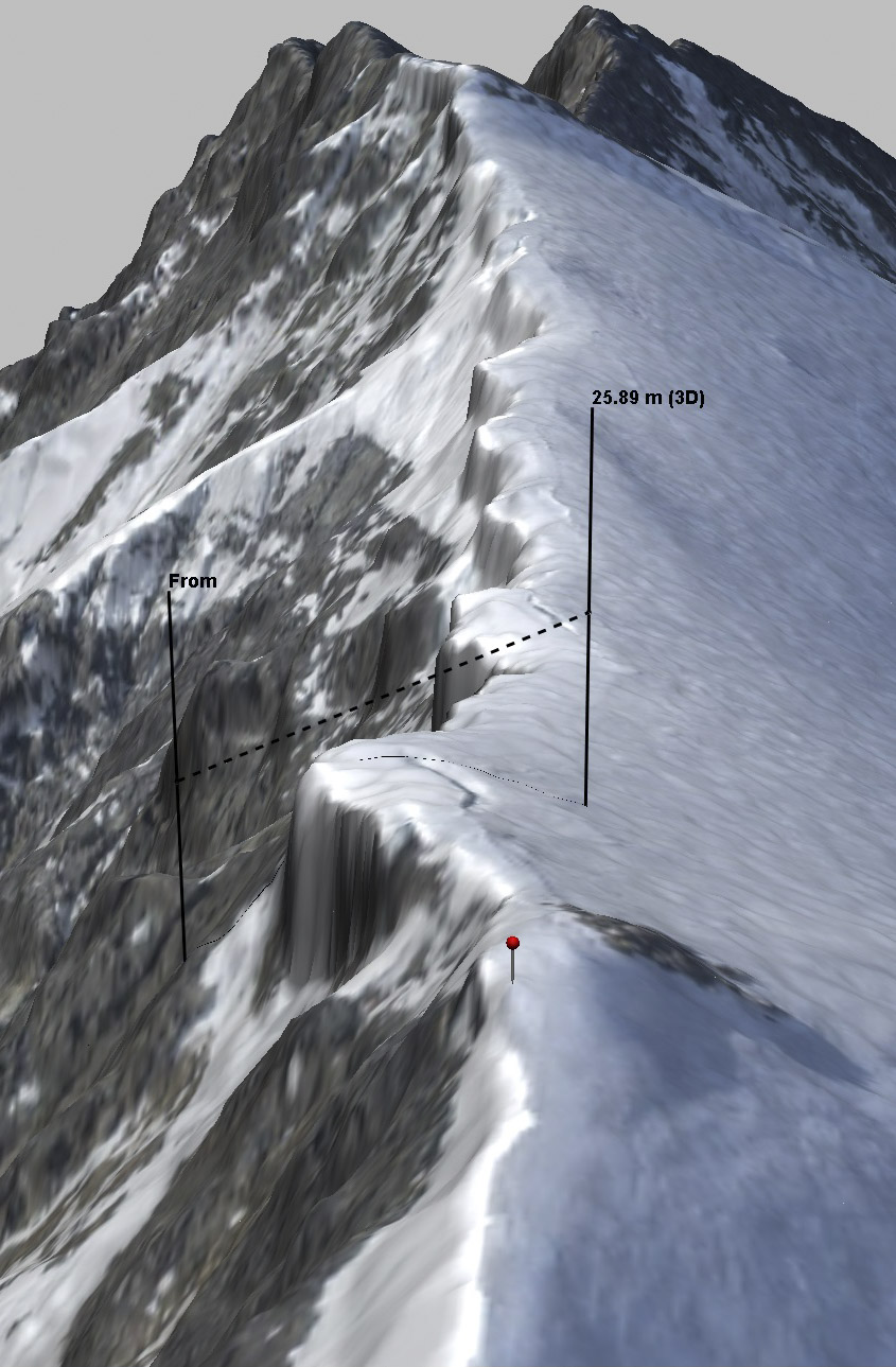
We hiked up several of the peaks to measure their height with GPS, shown here as yellow dots superimposed over the 3D visualization of fodar data. Static GPS occupation times were only 20 minutes or so, so accuracy for both static and kinematic points was only 10 cm or so, but nevertheless the hundreds of GPS measurements agreed with fodar to within a standard deviation of 10 cm. In practice, because the measurements were not made on the same days, some of the change is real, but we conservatively determined our precision in the mountains to be 20 cm at 95%.
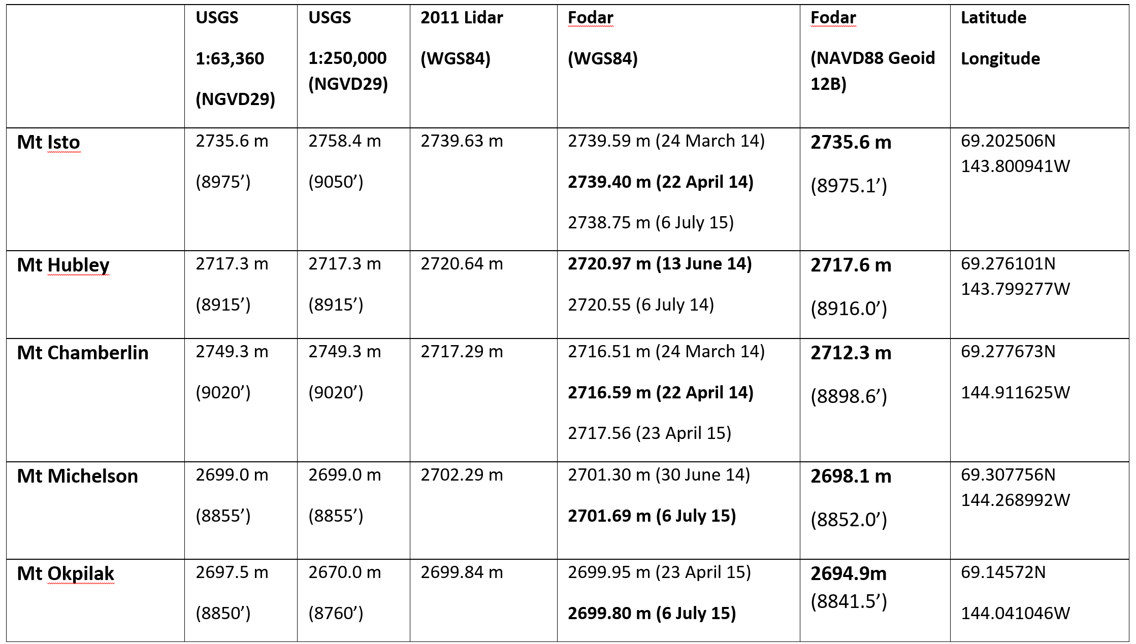
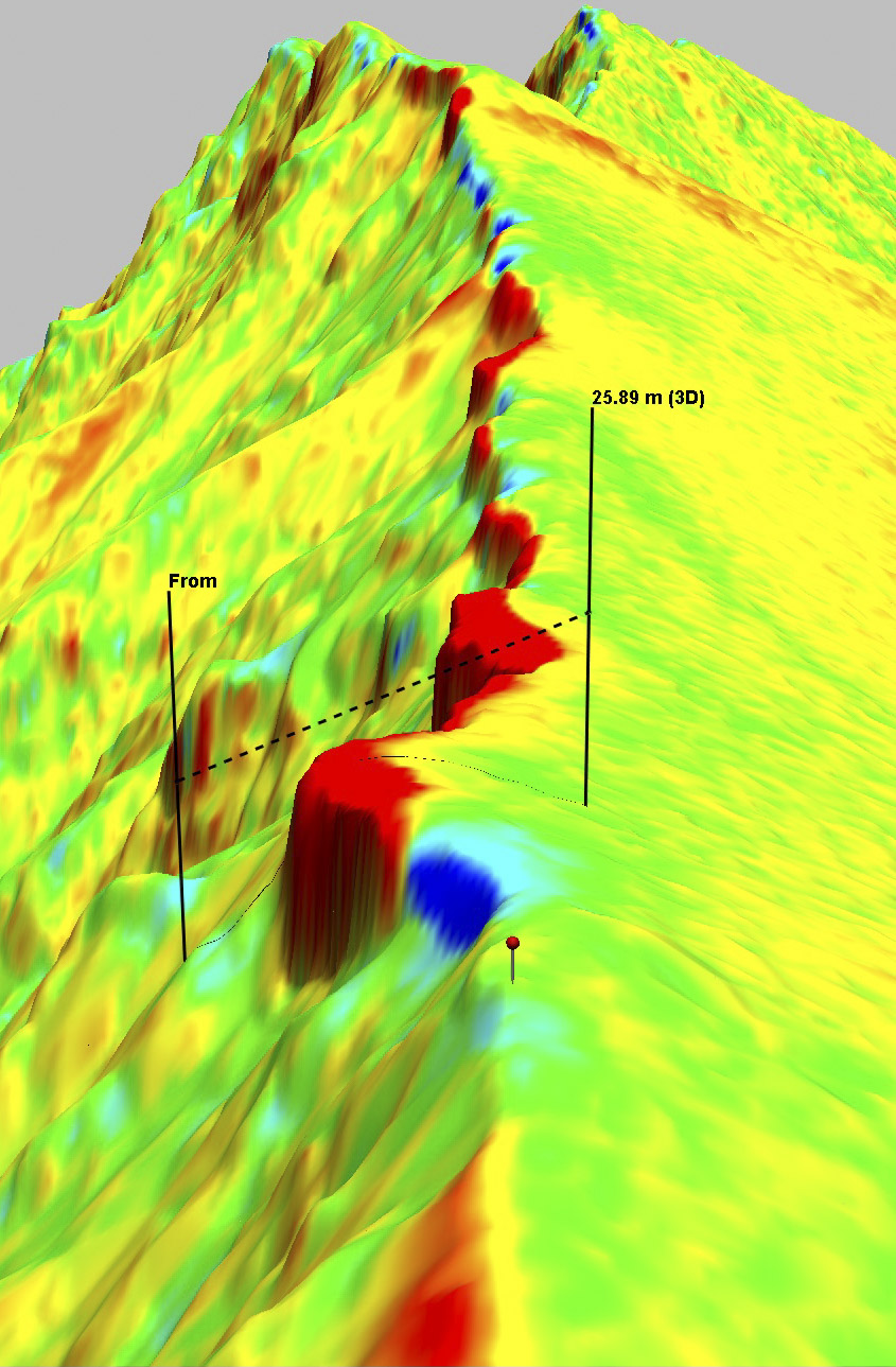
These are the results of our fodar measurements of the five mountain peaks in question. Here are shown 2-3 measurements each with fodar. The scatter for each peak ranges from 8 cm to 97 cm, with all but one below 40 cm. The challenge for precision validation is that the imagery clearly shows that much of the differences seen here are real — the peaks are capped with snow and ice cornices, which have changed in shape between the months and years between measurements. Nevertheless, analysis of these data show over bare rock show that the scatter reduced to better than 20 cm and that we can actually measure even subtle changes in steep snow packs, as shown below.
Here is a video of Mt Hubley’s fodar data. Note the high resolution detail and reality of appearance, qualitatively confirming what the quantitative validation studies have shown. I hope these videos will also help debunk the myth that fodar cannot measure snow and ice due to contrast issues, whether in shadow or bright sun. In terms of applicability to mountain measurements, also note that it takes an especially powerful and specialized lidar to fly above this terrain and get returns from snow and ice; because fodar is a passive measurement, I can fly at any height I like using the same inexpensive camera.
We found Mt Hubley to be the second tallest peak in the US Arctic. McCall Glacier lies in its northern shadow, a place I have spent more than 3 years of my life over 30 or more expeditions.
What can measuring Alaska coastal villages tell us about fodar accuracy and precision?
In 2015-16, I mapped about 35 villages on the west coast of Alaska as part of a complete mapping of the west coast. About two thirds of this was funded by the State who then validated them through comparison to professionally-surveyed GCPs, along with my own assessments. Both assessments showed vertical accuracy of about 10 cm and vertical precision of 10-16 cm, and a perfect (subpixel) horizontal accuracy.
You can find their report here or in the window below.
[pdfviewer width=”800px” height=”849px” beta=”false”]https://fairbanksfodar.com/wp-content/uploads/2018/02/dggs_village_report.pdf[/pdfviewer]This is the official State report on these data. Below is Table 2 from that report, which shows their independent assessment of the accuracy and precision of these data.
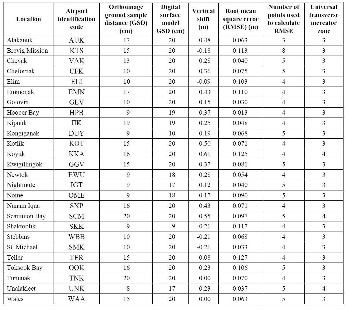
Above is the State assessment of accuracy and precision of the village data. The “Vertical Shift” of the 5th column is essentially the accuracy of the data set when no ground control was used. The precision after this shift reduced the GCP misfit to zero, roughly twice the values column 6, ranged from 6 to 24 cm, with a final 95% value of about 16 cm. Note that these values are based typically on only 4-5 check points per village.
You can find an interrim report of mine here or in the window below that gives lots of visual examples of the data to reveal its quality and its noise.
[pdfviewer width=”800px” height=”849px” beta=”false”]https://fairbanksfodar.com/wp-content/uploads/2018/02/fairbanksfodar_november_report_151130b.pdf[/pdfviewer]Here is an interrim report of mine, at the time when I had submitted the data for review. Here you will find not only a complete accuracy assessment, but visual examples from each of the villages detailing data quality and any noise found.
You can download or view the data online here and then fool around with it yourself. Be sure to turn off all other layers than “SfM”, then zoom into the west coast to find the village outlines.
You can find a blog which discuss the accuracy and precision of these data here or links to all of the blogs for this project here.
These data are now being used by the State to produce a beautiful set of colored-coded risk flood and planning risk maps for each village which you can find here.
These data are also now being used to help with flood inundation mapping. The basic idea is that villagers take photos of their village during a storm when the village is flooding, then these water-lines found there are matched up to my orthophotos. Then the corresponding elevations are extracted from my DEMs to produce an elevational map of inundation for that particular storm, which can then be used for future planning as well as for improving predictive modeling of yet larger storms there and elsewhere. You can find a paper written by the State on this here.
[pdfviewer width=”800px” height=”849px” beta=”false”]https://fairbanksfodar.com/wp-content/uploads/2018/02/dggs_storm_photos.pdf[/pdfviewer]
What can measuring Alaskan beaches tell us about fodar accuracy and precision?
In addition to the study shown above on coastal villages, I also mapped about a mile-wide swath of the west coast of Alaska, as well as some of the Arctic Ocean coast. The west coast data stretch about 2000 miles long, roughly the same as the east coast of the continental US, so this presents a unique opportunity to test the data accuracy and precision of the data across huge spatial scales. For the portion of the data from Wales to Bethel, the State contracted for new professionally-surveyed ground control and check points. I used none of these in processing, so from the fodar perspective they were all check points. I found all of the data within the vertical specifications and so did not shift the data, primarily because I felt this ground control was insufficient to warrant such shifts, even though the misfit between fodar elevations and control were often in the 20-30 cm range, with a few even higher. That is, as I have been arguing, as accurate as the GCPs are, I believe ~60 of them are insufficient in amount to shift over 100 billion pixels, especially as some of these were not photo-identifiable, were on rocky points or cairns, or were on the center of plates which did not sit flush with the lumpy tundra. Further, comparing this coastal fodar to the villages shown above, which often use the same photos and air control, show the differences between the shifted village data and the coastal data to be within 10 cm generally of many millions of pixels. I weight these comparisons much more highly, for the reasons given previously.
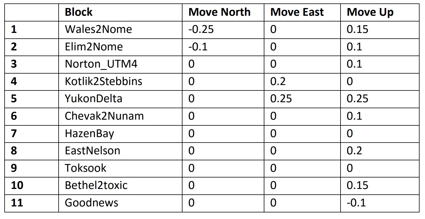
This table from my final report shows the results of my accuracy assessment, based on both GPS survey points and repeat mapping. They are all well within the specifications for the project so I did not shift these enormous data to improve their accuracy, preferring to wait until we had larger sections of repeat mapping to use to ensure the shifts would actually lead to increased accuracy. In any case, you can see the shifts are all quite small; that they mostly all suggesting moving the fodar up could be real, or could be related to a bias caused by surveyed points often being a bit higher than the surrounding land. The 11 blocks are stretches of coast 50-200 miles long processed as independent blocks, with the blocks in order from north to south and given names related to villages or features en route.
Here you will find my full report, as well as in the window below. It contains dozens of visualizations of the data, revealing both its quality and its errors; note that these visualizations are arranged on the page such that one can flicker between the DEM and ortho by flickering page-to-page, so opening in your own viewer and setting the view to an entire single page rather than scrolling between pages will optimize viewing experience. Generally speaking, the gaps amounted to much less than 1% of the coverage and the errors were confined to the bonus data. The bonus is the data outside the range of the specification of 1500 m inland, which I delivered because it is still great quality and useful, it just has the normal artifacts of edge data. Here you will also find all of the ground control and check points, shown as a photograph in the field with an associated screenshot of the data. I suspect this is the most comprehensive review of SfM photogrammetry ever undertaken, if only because this is likely the largest such mapping project ever undertaken. See in particular Table 2, which gives a summary of all of the quantitative means I used in this analysis. These data were delivered in July 2016; as of February 2018 only some of these data are online here at the State’s site but the remainder should be online shortly.
[pdfviewer width=”800px” height=”849px” beta=”false”]https://fairbanksfodar.com/wp-content/uploads/2018/02/ff_dnr_finalreport_wfigures_160728_opt.pdf[/pdfviewer]This is the accuracy and precision report I submitted with the data in July 2016. The State is still working on publishing its own assessment; it should be out soon and when it is I will include it here. In the meantime, I do not think you will find a more comprehensive study of fodar accuracy and precision than you will find in this report.
What can measuring road surfaces tell us about fodar accuracy and precision?
Roads present unique challenges and opportunities for fodar, both in terms of application and validation. I’ve mapped the entire Dalton Highway several times and pieces of it many times, the entire Richardson Highway, and many other smaller segments of roads for our DOT. Unless I’m mapping locally here, I typically employ a budget form of budget fodar for roads. Traditionally, one flies rectangular blocks of lines over the turny-twisty road, but rather I fly one line up and one line down, following the twists and turns. Two lines are really the minimum for accurate fodar, so that the bundle adjustment has enough information to determine tilts of the photos, but more is better up until about 5 lines. But flying a road 3 times leaves you at the wrong end of it, and 4 lines or more drives up costs considerably, especially if it pushes you into a multi-day acquisition. Because roads are one of the few places in Alaska you can drive to …, it presents a great opportunity for collecting gobs of economical ground control, especially when you are working for surveyors. The data I have delivered thus far have been accurate enough for their intended purpose, but in collaboration with DOT our goal over the next year is to use these 8-10 data sets to assess the limits of the budget budget technique and see if we can push them further by tweaking methods, such as perhaps by adding a few GCPs into the bundle adjustment. Potentially we have hundreds of ground control points to use in these validation studies, the real challenge is selecting appropriate check points to validate at the centimter level because most of these points were not collected for the purpose of being identiable in such high resolution imagery. When care is taken to select only the best of such points, we get numbers like 30 cm for horizontal accuracy and 10 cm for horizontal precision (95% RMSE) for 8 cm GSD and 8 check points, but elsewhere on that same project when 180 check points were used the precision dropped to 40 cm (95% RMSE); however the picking accuracy (that is, selecting the point on the ortho that represents the field measured point) was only about 2 pixels and sometimes worse. That means that validation is something like 40 cm +/- 20 cm, but even this range does not capture what we get when choosing points more carefully. So most of these points are better for checking vertical accuracy and precision, which is something we have not done yet rigorously in this context. Given the data in hand and that it is on the road system, we have the opportunity to use the orthoimage itself to select check points in the field that we are sure can be determined to within 1 pixel on the ortho and given on-going needs for road maintenance we have opportunities for repeat mapping both for change-detection and for validation. I’ve been mapping river ice using this same two-pass technique several times per year for several years now as part of this study, which has shown the precision in the overlapped area to be in the same 10-20 cm range as all other studies have shown, allowing us to measure vertical bulges of river ice of only 10 cm as slugs of water move past it, and I expect the road studies to be no different. So these road validation studies are just beginning, and expect updates to this section of the page. In any case, the data have already proven quite useful, with estimates of 6 figure savings compared to traditional field surveying which, rather than putting State surveyors out of work, keeps them busier than ever because they can cover greater ground in summer by reducing their field time at each site and those that would normally get laid off in winter when no surveying is done can stay employed through the winter ‘surveying’ on the computer screen by extracting from the fodar data the measurements they normally would have collected in the field, so its a win-win for everyone I think.
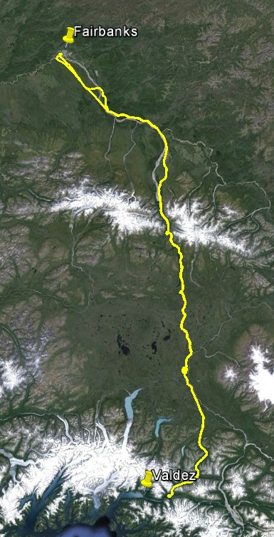
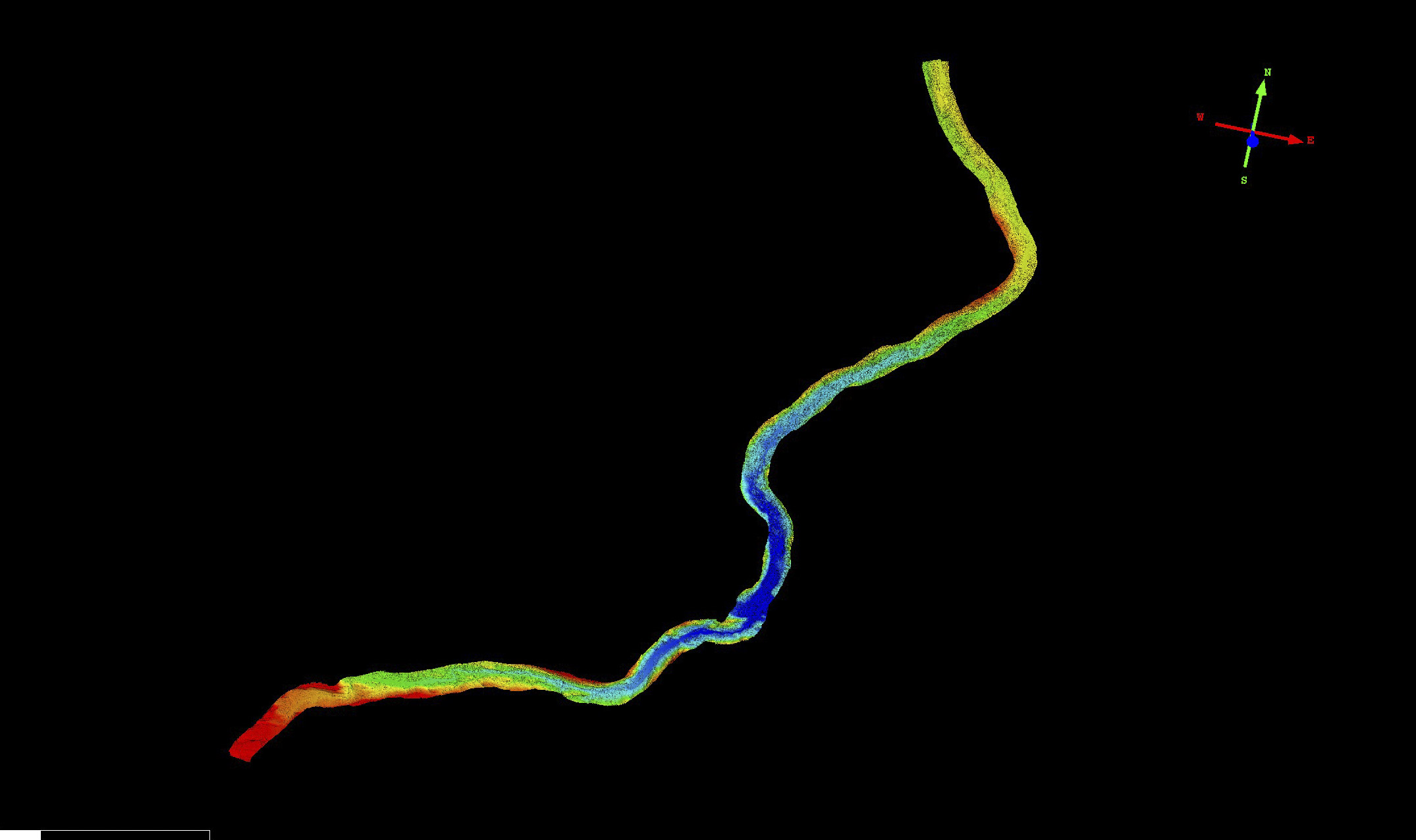
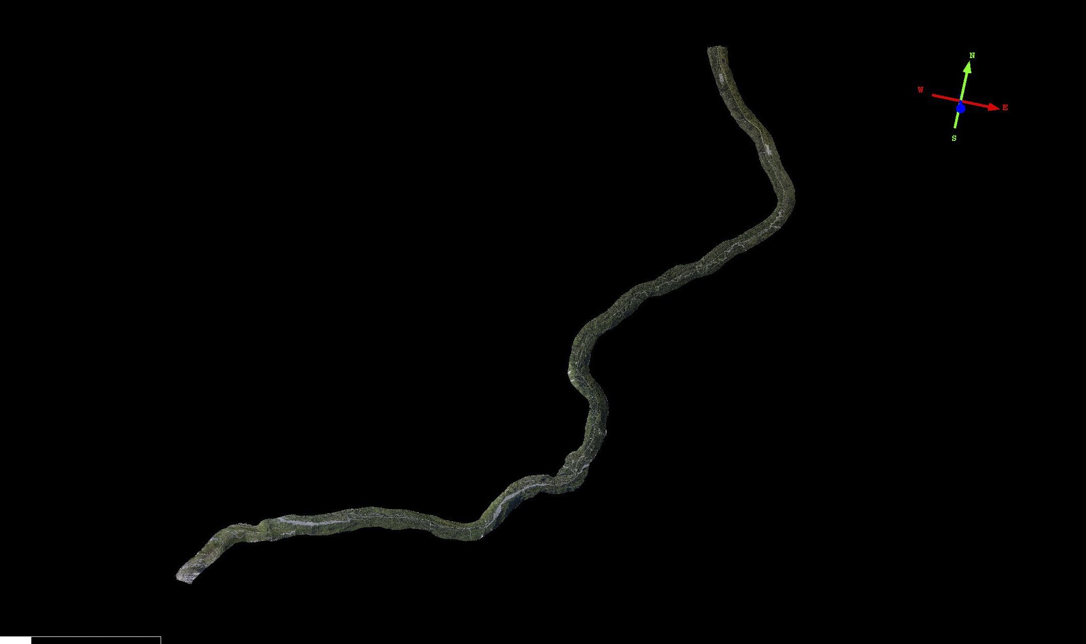
Here is an example of the two-pass method, mapping the Richardson Highway. Flying a third line would leave me in Valdez and a fourth would turn this into a two day project which, given the three weather systems involved, could turn that into a two week project. That is, an important variable in saving money is minimizing not just the flight time but optimizing flight time for likely weather windows. I’m planning to map this highway again this summer to measure displacement across the Denali Fault, which runs through the Alaska Range. That is, I believe the data are accurate enough to measure the 4-6 cm per year motions of the tectonic plates here.
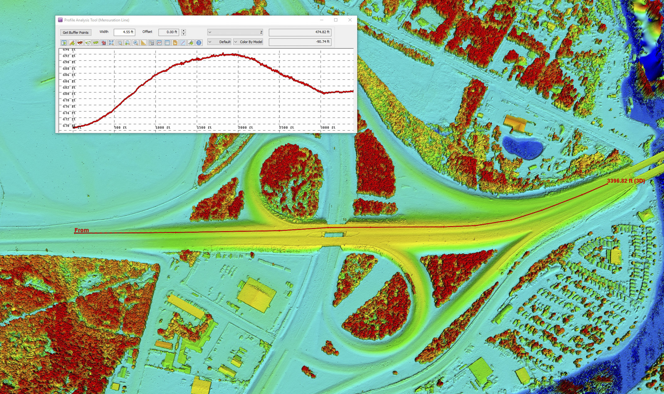
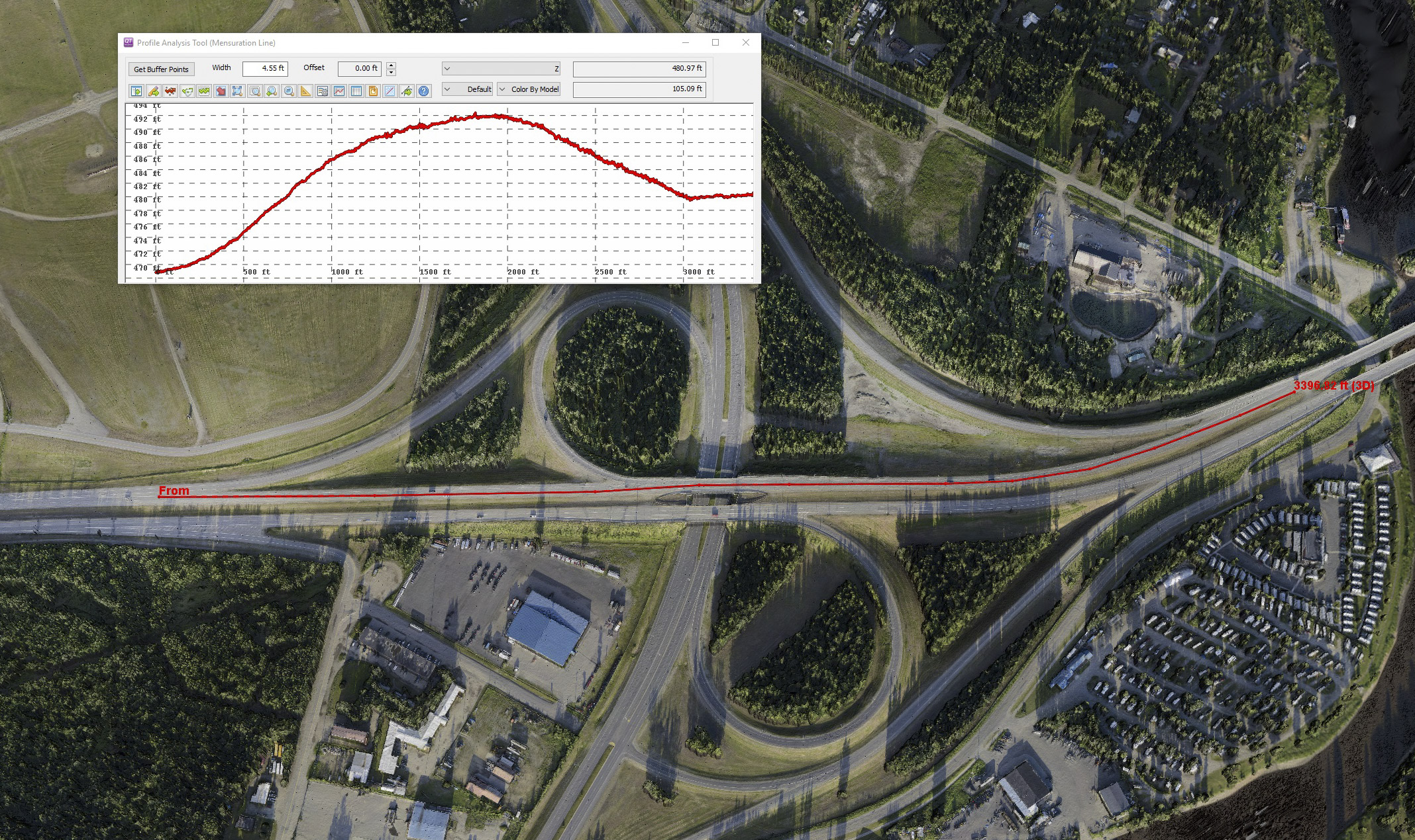
Here is an example of a typical check point. This is how the point fell onto the orthoimage with no shifting. It looks great, but we cannot tell to within better than 1-2 pixels at best how accurate the data are. Worse, it’s not clear which part of the feature was measured in the field as there are no corresponding photos. So to get the most out of a validation study, we need to select GCPs with photo-identification at the subpixel level in mind and compare these results with repeat-maps which give us millions of such comparisons. Higher resolution data could also help and is easily done, but there is a trade-off with file sizes becoming even more enormous for roads 100s of miles long, as well as the ever-present question of how accurate is accurate enough to answer the questions being asked. It would also seem that these data pay for themselves in validating the field measurements (the opposite of the studies on this blog), such that it can very easily determine when field notes or metadata place the field point in the wrong location.
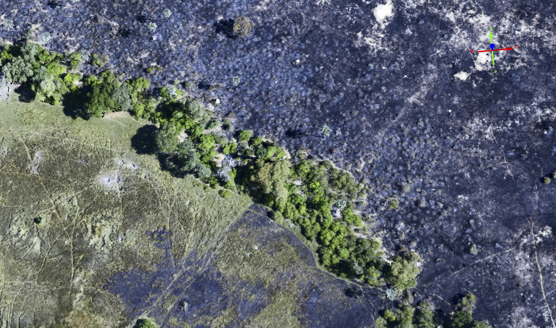
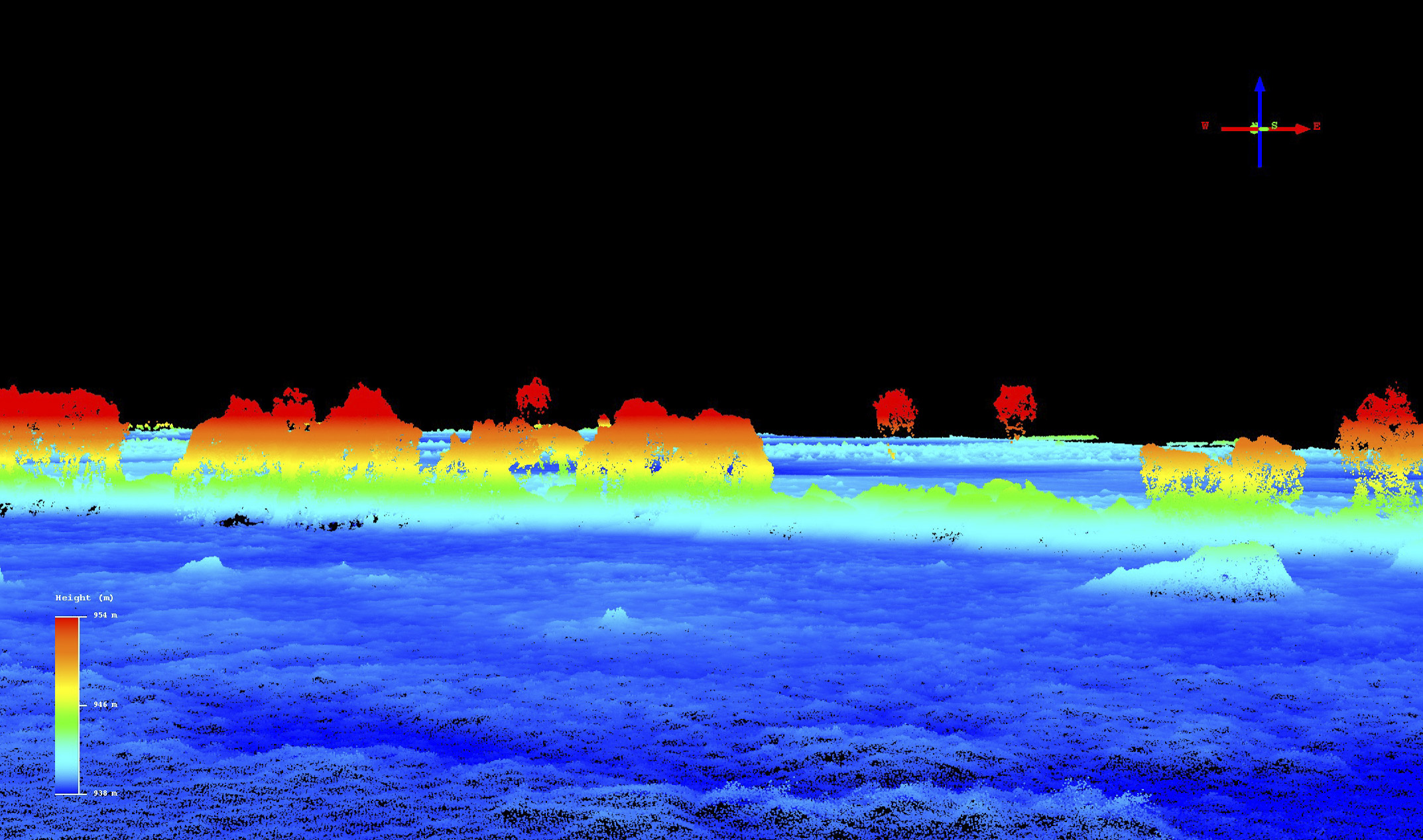
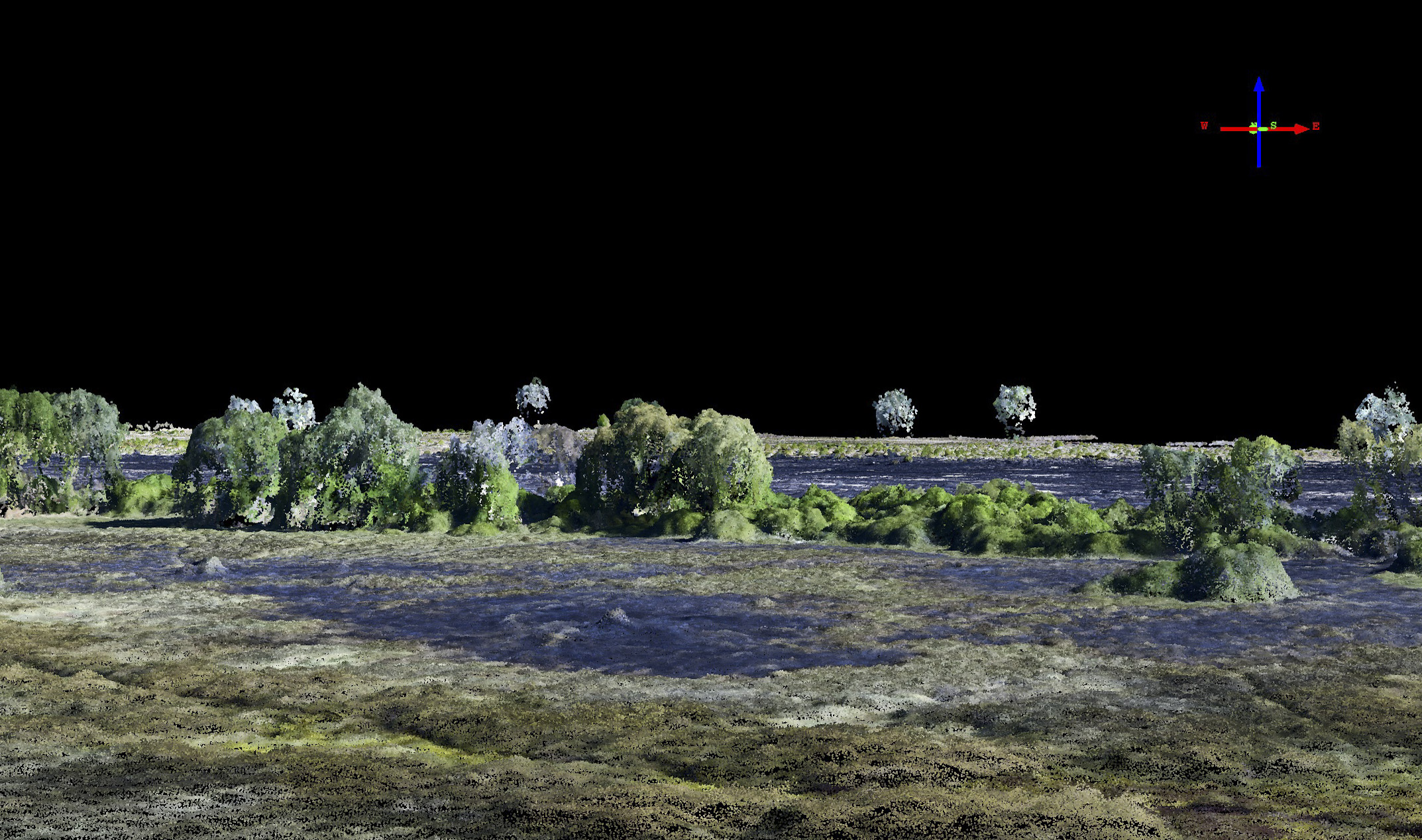
What can measuring forests in Botswana tell us about fodar accuracy and precision?
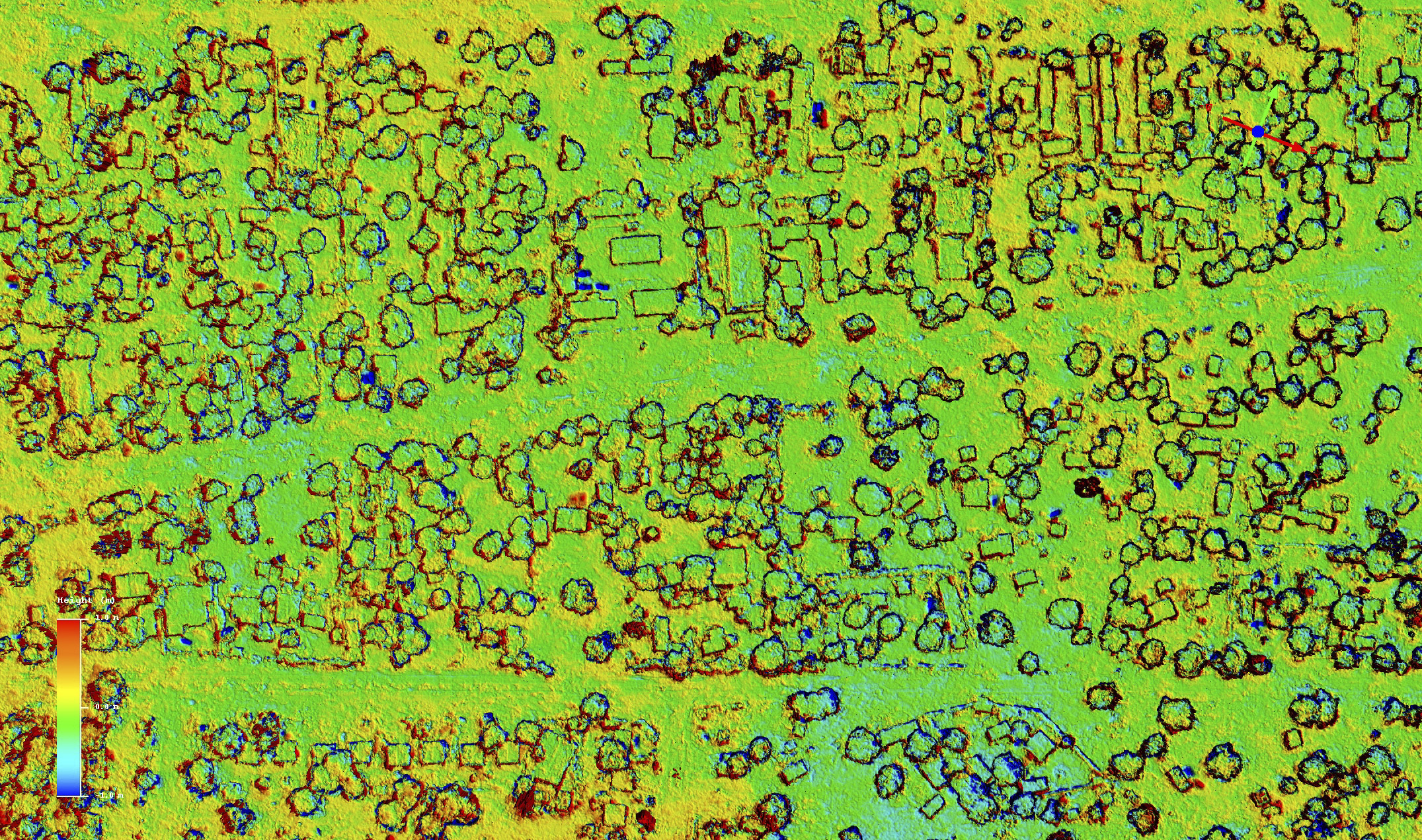
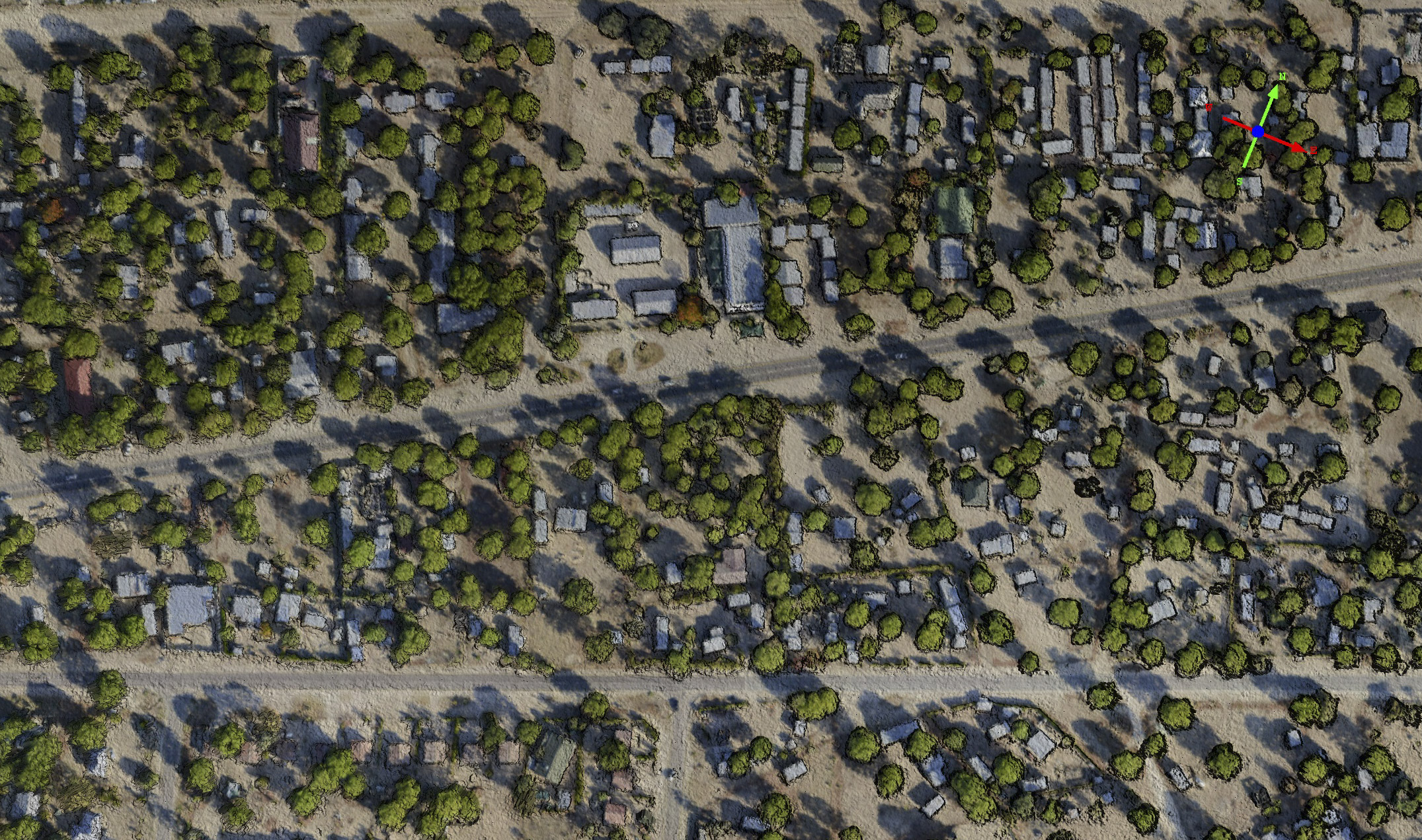
Mapping vegetation and canopy heights, or under them for that matter, has not been a priority of mine as I tend to focus on Arctic subjects, but as I start to do more of this work I’m starting to also focus on understanding the accuracy and precision of those targets. Recently I spent some time in Botswana mapping elephant habitats and how they are changing over time, so we also now need to understand how small of a change in tree canopy we can expect to measure reliably. I did this by mapping the Maun, Botswana, airport area twice, on two separate days, as this area has a nice mixture of hard surfaces (the runways) and suburbs with trees, houses, cars, etc. Below are a few examples from that study, but you can read the full blog here. We will be returning there shortly to re-map the larger transects to look for change (and further assess accuracy) and add some new transects. As many people think fodar cannot map trees for some reason, I have included a number of videos below of the fodar point clouds which I think give a great sense of how we can map trees using this technique. But as the image pair below show, fodar accuracy in the trees is about the same as it is for everything else.
So what’s the bottom line?
Here I have tried to capture accuracy and precision of fodar data across the full range of possible targets in Alaska. These rigorous studies have been conducted on nearly flat terrain to show that repeat-mapping can measure even the thinnest of Arctic snow packs, on some of the steepest terrain in Alaska, and on continental scales covering the west coast of Alaska. I’ve also demonstrated fodar’s ability to map trees and the ground beneath them with an example from Botswana. In all cases, the accuracy and precision of these data, without use of any ground control, is better than 30 cm at 95% RMSE using the best validation methods available, including comparison to GPS surveyed ground control, to other fodar maps, and to lidar maps. When some ground control is utilized, the accuracy drops to the precision level, which is typically in the 10-20 cm range at 95% RMSE. There have been other studies not shown here that show essentially the same results, and as new ones emerge that add some new twist or rigor I will add them to this blog. In the meantime I invite you to dig into these analyses and give me any feedback you care to share or ask any questions you may have.