First Results from 2018 Botswana Fodar of Elephant Habitats2019-03-162019-03-19https://fairbanksfodar.com/wp-content/uploads/2014/09/fodar_logo4mn.pngFairbanks Fodarhttps://fairbanksfodar.com/wp-content/uploads/2019/03/img_9877_acr-3.jpg200px200px
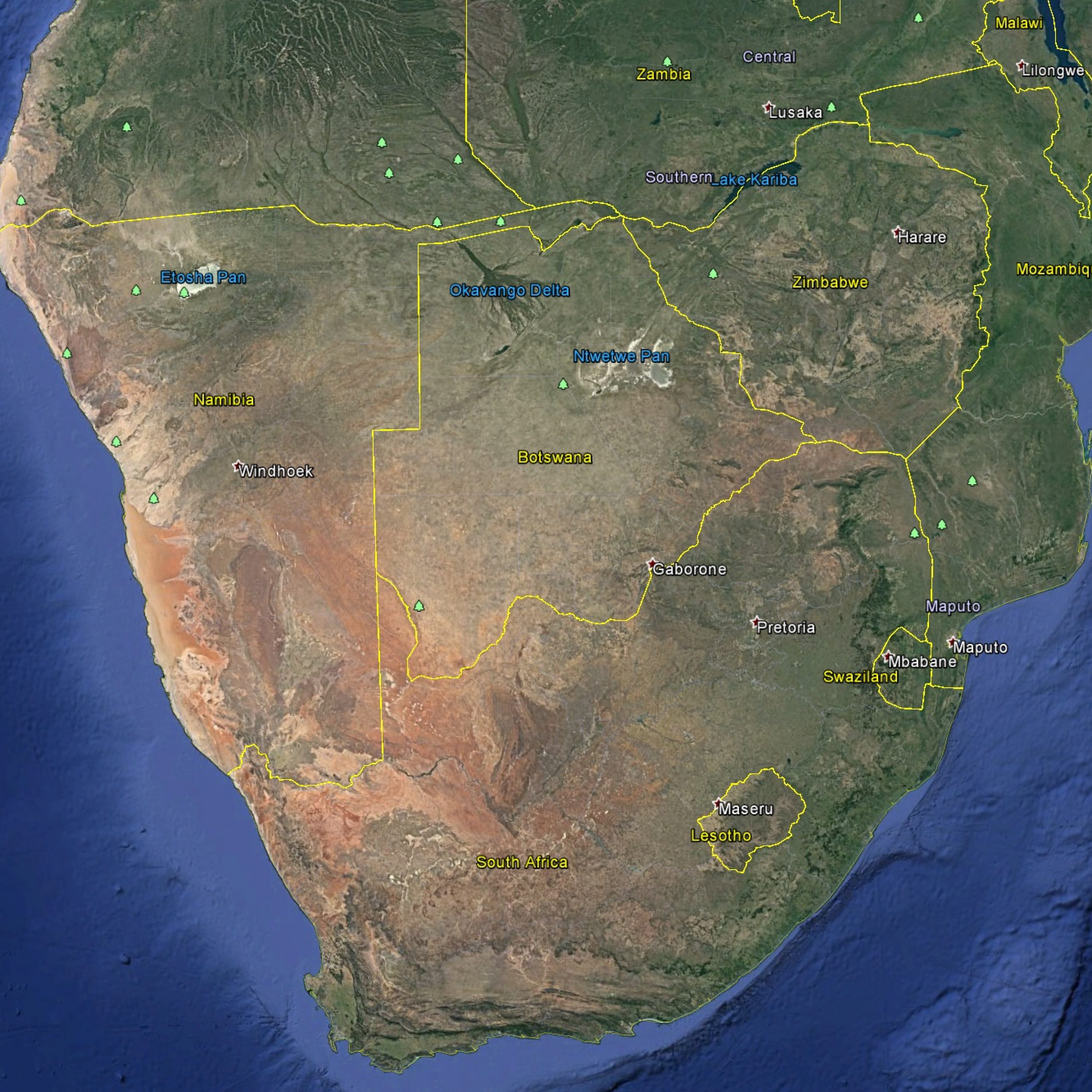
We spent most of November 2018 in Botswana studying elephant habitats using fodar, expanding on our work in 2017. This blog summarizes our 2018 mapping work from acquisitions to data validation, as well as some samples of the analyses we hope to accomplish with it. In addition to making maps, we also learned a lot about the local ecology, some of which Turner shared here.
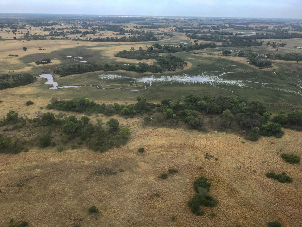
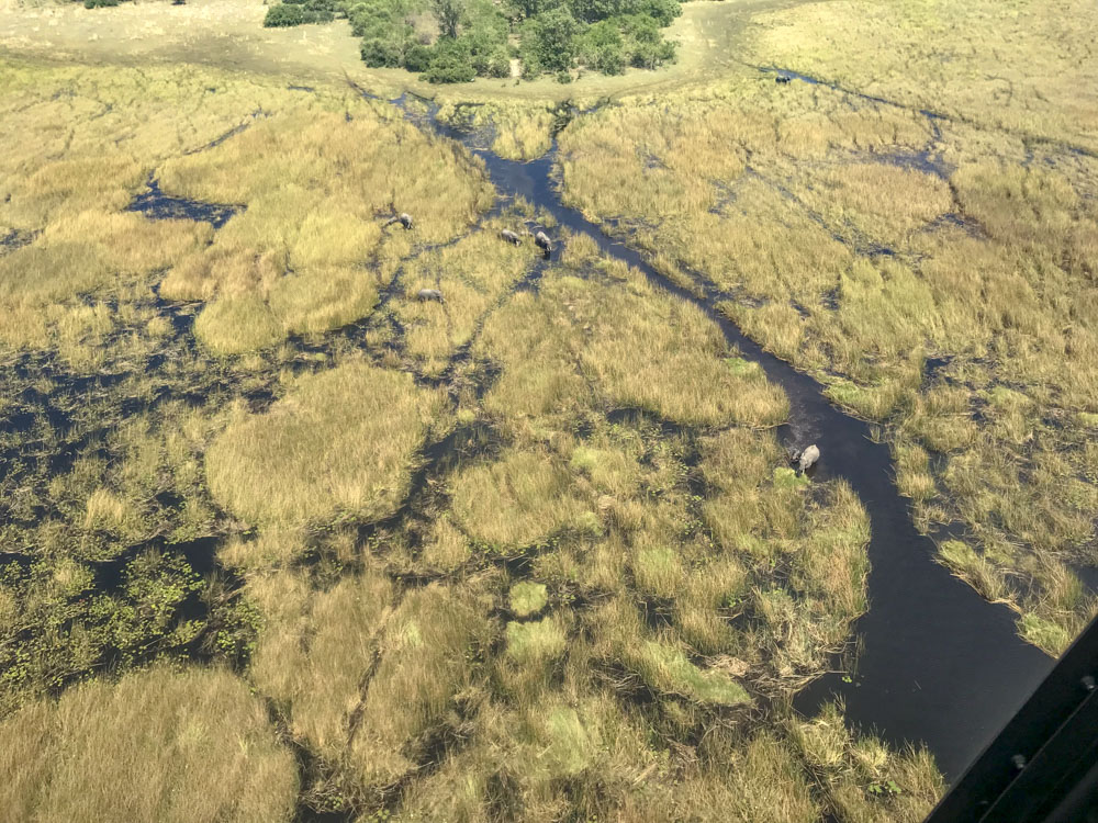
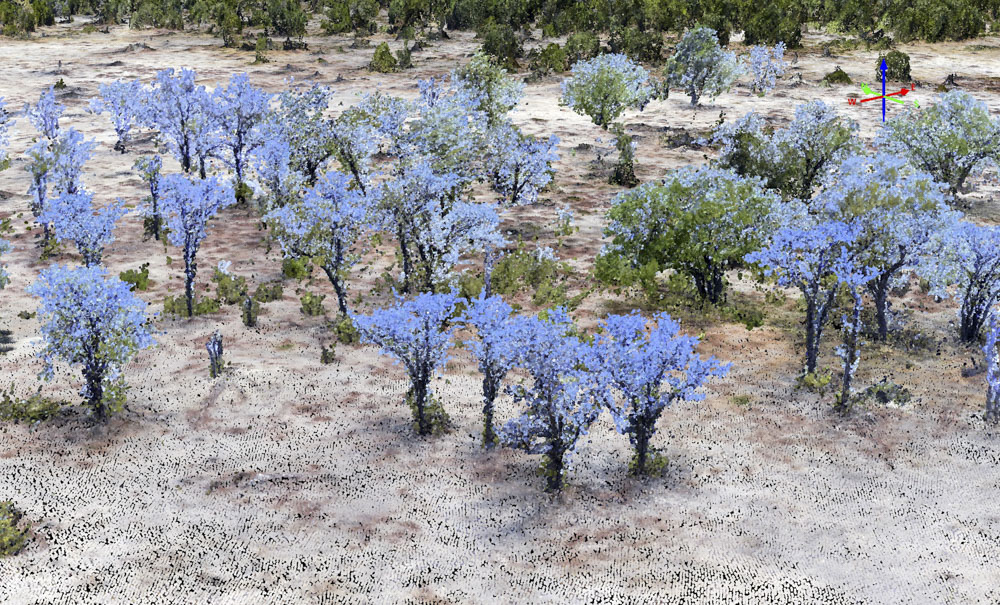
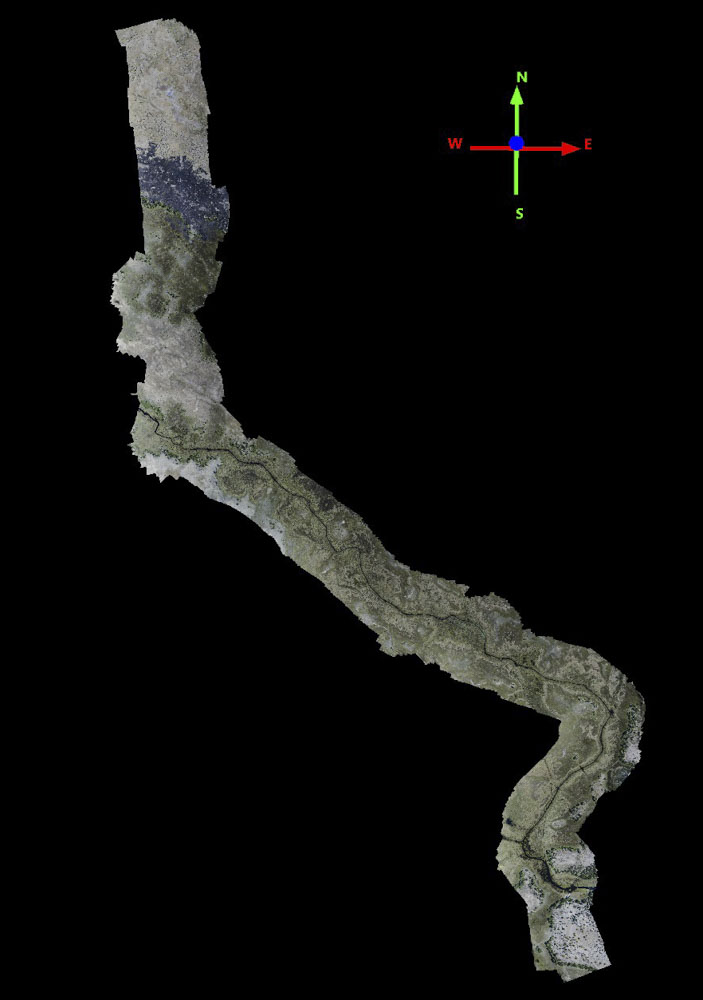
Here is a 3D visualization of the fodar data we acquired in 2018, showing vegetation alongside a river leading into the Linyanti swamp. Note that you can not only determine tree size and shape but distinguish tree species, even if you are not a tree expert. Note also that not all of the trees have leaves yet, the rainy season was just beginning during our stay.
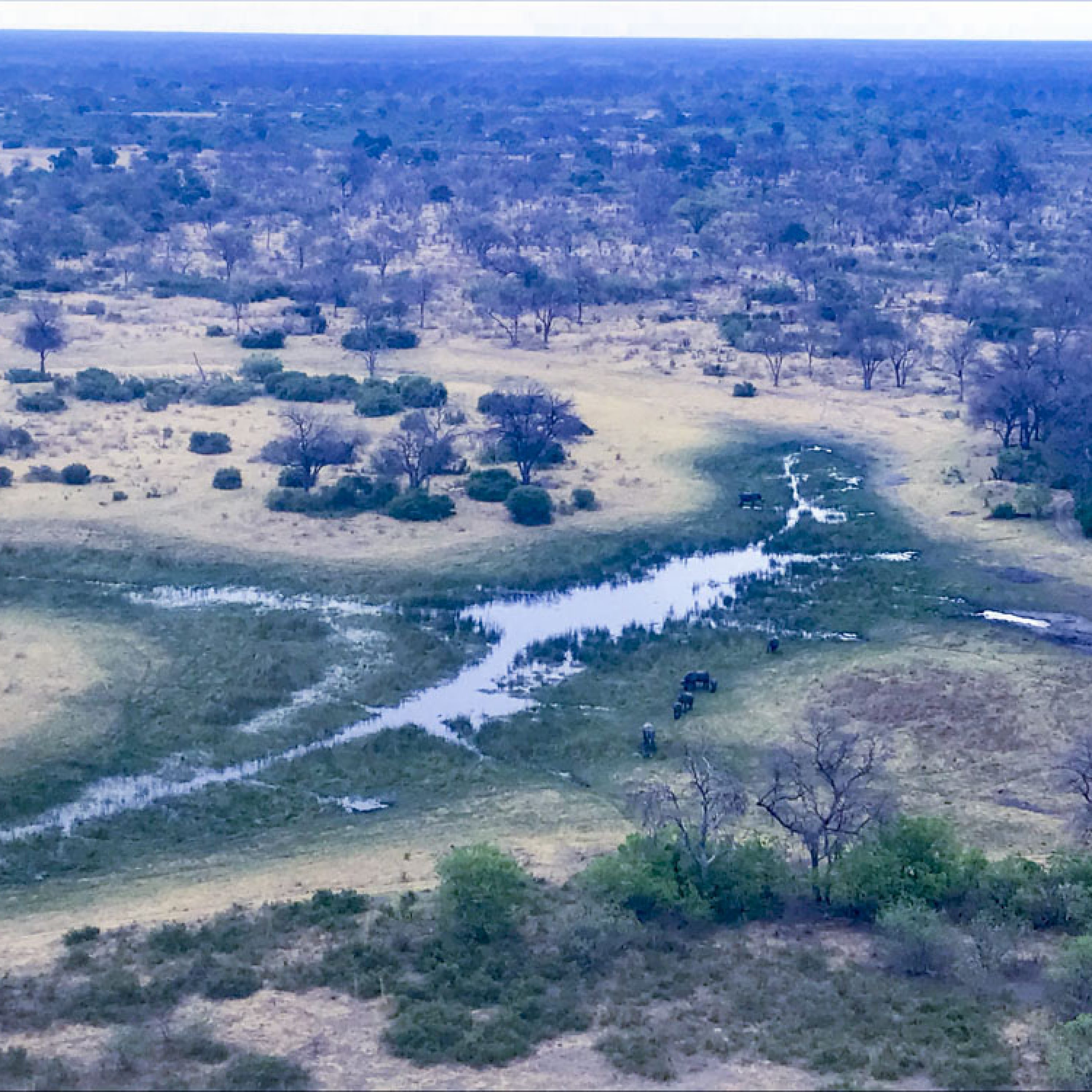
Here is a 3D visualization of the 2018 fodar data alongside the Linyanti swamp. Here you can not only see and measure the variety of woody vegetation that grows here, but also the extent, size and species of swamp grasses and floating vegetation. Anything on the landscape becomes part of our maps, including elephant trails through the swamps or 4WD truck trails over the ground.
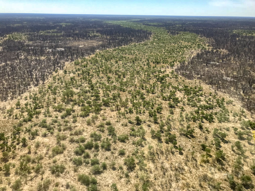
Here is a 3D visualization of the 2018 fodar data flying us from the Linyanti swamp into the Savuti Channel, a fascinating drainage feature with millions of years of interesting tectonic-hydrologic history to explore. Note how well the water itself is resolved due to the floating vegetation, such that we can easily measure water levels and gradients.
Our work is focused on understanding the impacts of elephant browse on woody vegetation. Woody vegetation here basically means trees and things that would like to be trees except that elephants keep eating them or knocking them over. Foraging elephants exert a primary control on the distribution of woody vegetation and grasslands throughout the savannas of Africa, and have for millions of years. The mix of woodlands and grasslands, in turn, controls the distribution of related plant communities and the creatures that live there. So elephants exert a large control on the overall and local biodiversity by knocking over trees, munching on branches, and pulling up seedlings.
Here is a video from a documentary (The Great Rift: Africa’s Wild Heart, Episode 3) I recorded using my phone that nicely describes the impact elephants can have on woody vegetation. Episode 3 is a great way to learn more about the influence of elephants on biodiversity of the savanna.
Here is some video I shot with my phone showing a small herd of elephant knocking down trees, eating grass and seedlings, and strips leaves from branches. One thing I found interesting is that after knocking off large limbs, they didn’t spend much time with newly-accessible leaves. Our campsite is just behind the tree they knocked over; we had encounters this close probably 5-10 times per day on our game drives, giving us lots of opportunities to study their behavior.
Our hope is to get a better handle on the spatial patterns and temporal trends of the impacts elephants have on trees so we can track those impacts over time. For example, field studies have shown that woody vegetation gets taller the further you get from the major swamps (the Okavango and Linyanti in this case), presumably because the elephant populations concentrate around those swamps so have a greater impact on those trees closest to the swamps. So we hope to document whether this trend exists and can be monitored over large areas using fodar. As another example, speaking as a glaciologist pretending to be an ecologist, it doesn’t seem clear if anyone really understands how many elephants can live in Botswana before the woodland-grasslands balance they maintained for millenia changes due to over- or under-population of elephants, with a corresponding ripple effect on biodiversity. I think in Botswana a big long-term question is whether populations are increasing due to the elephants figuring out that Botswana is safer from poaching than in several of the surrounding countries. Trying to count them from the air is one method of figuring this out, but perhaps mapping the changes in forests is another; that’s something we will hopefully find out soon.
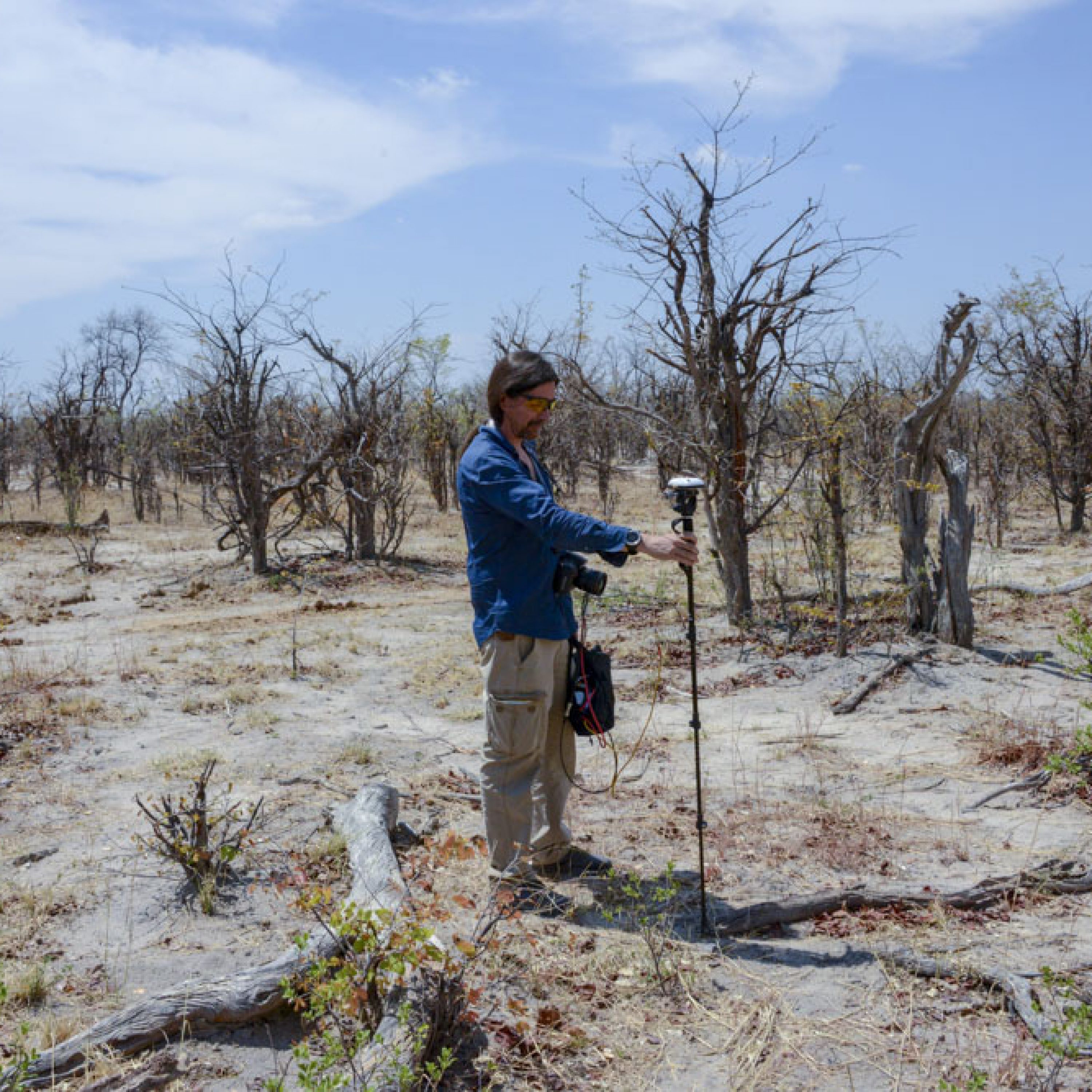
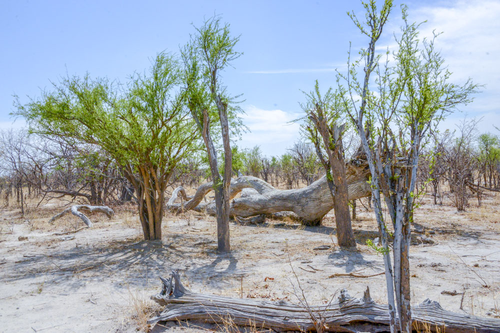
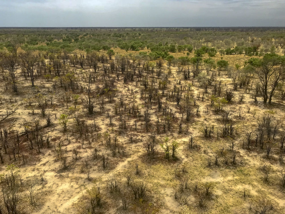
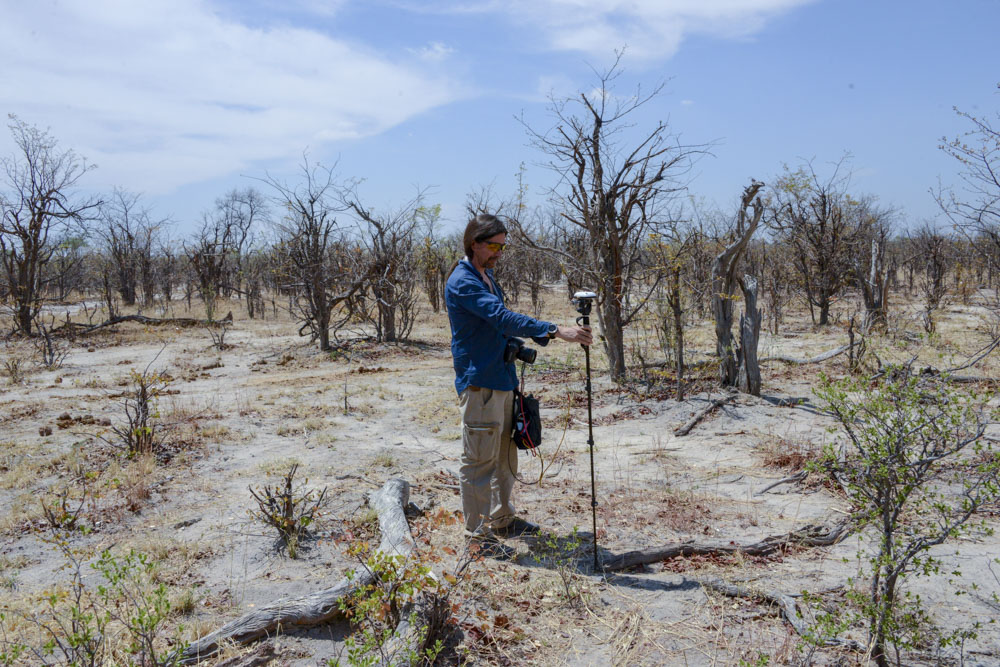
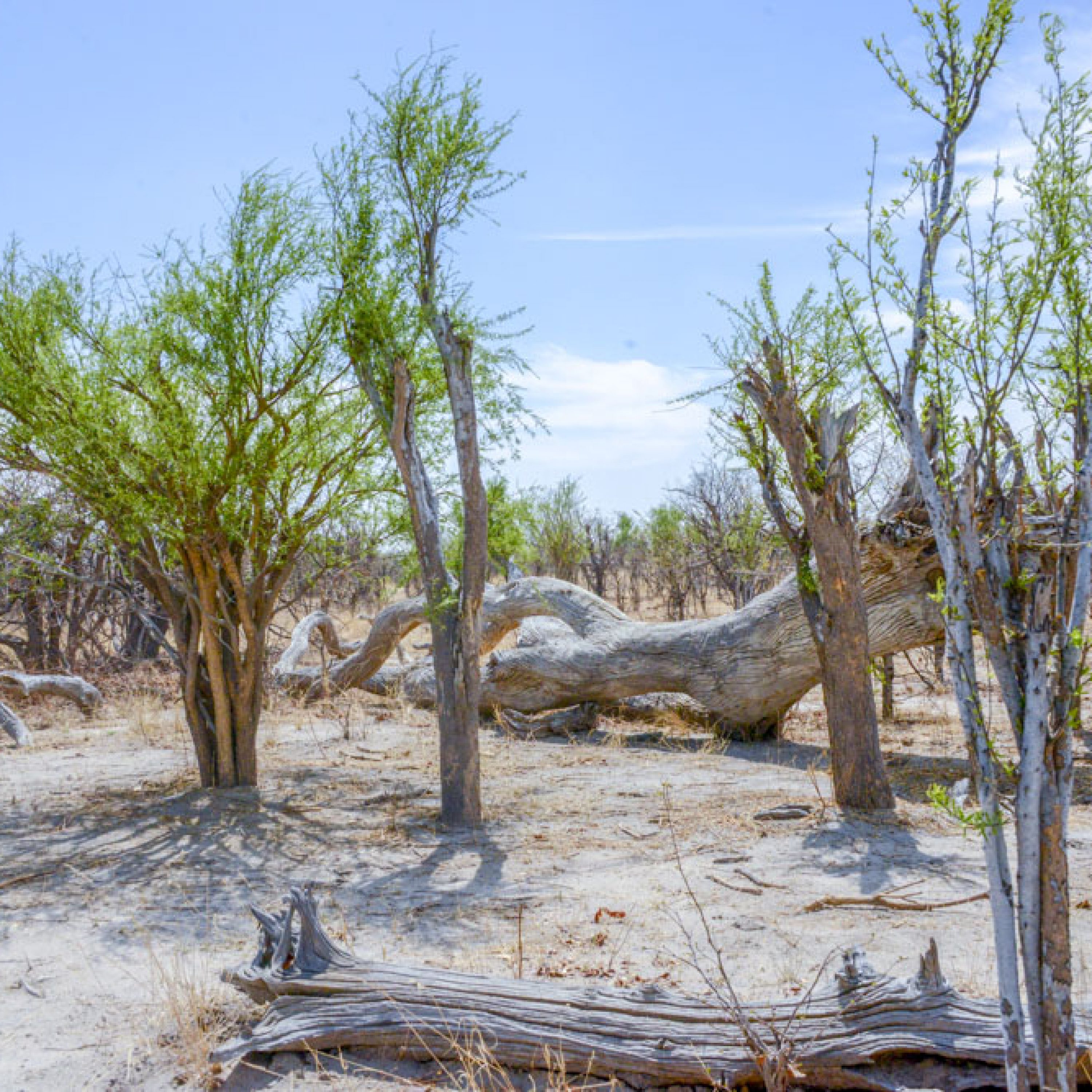
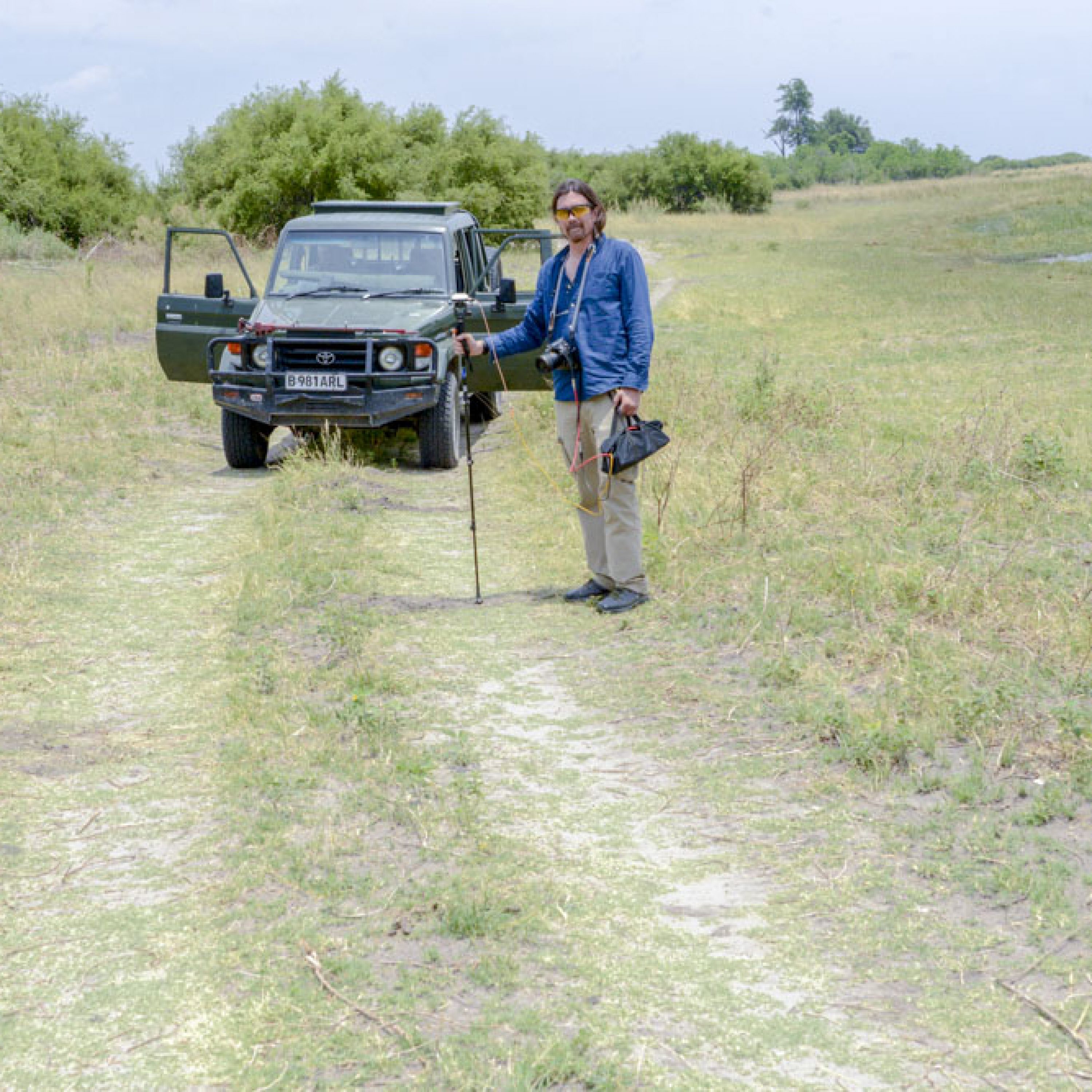
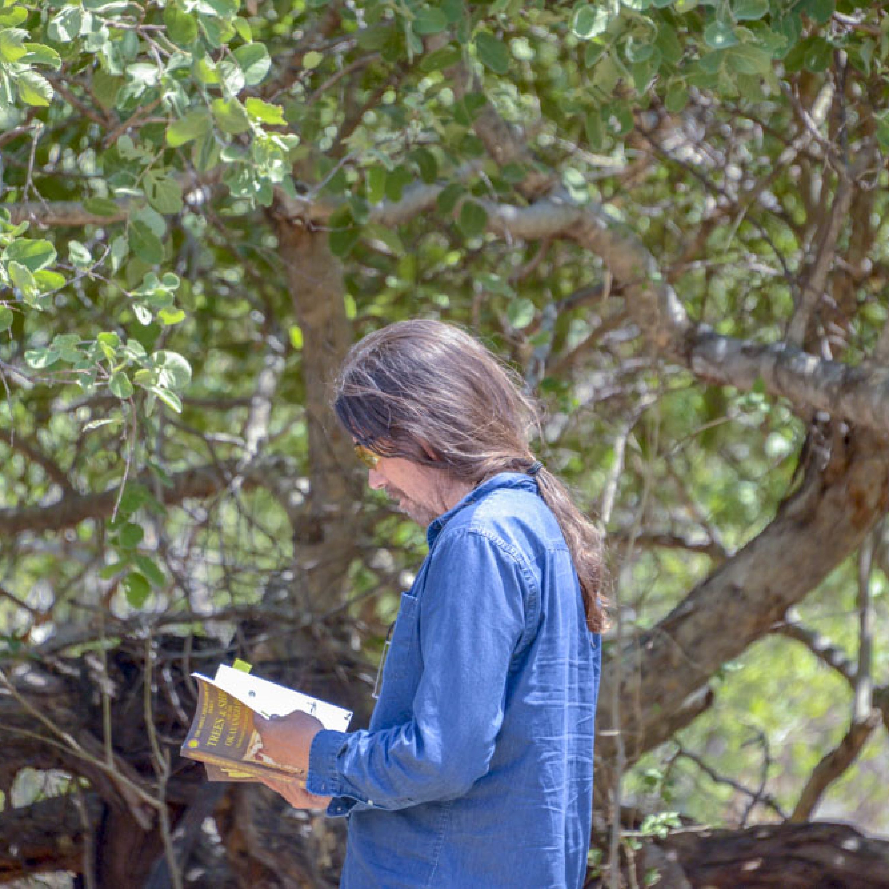
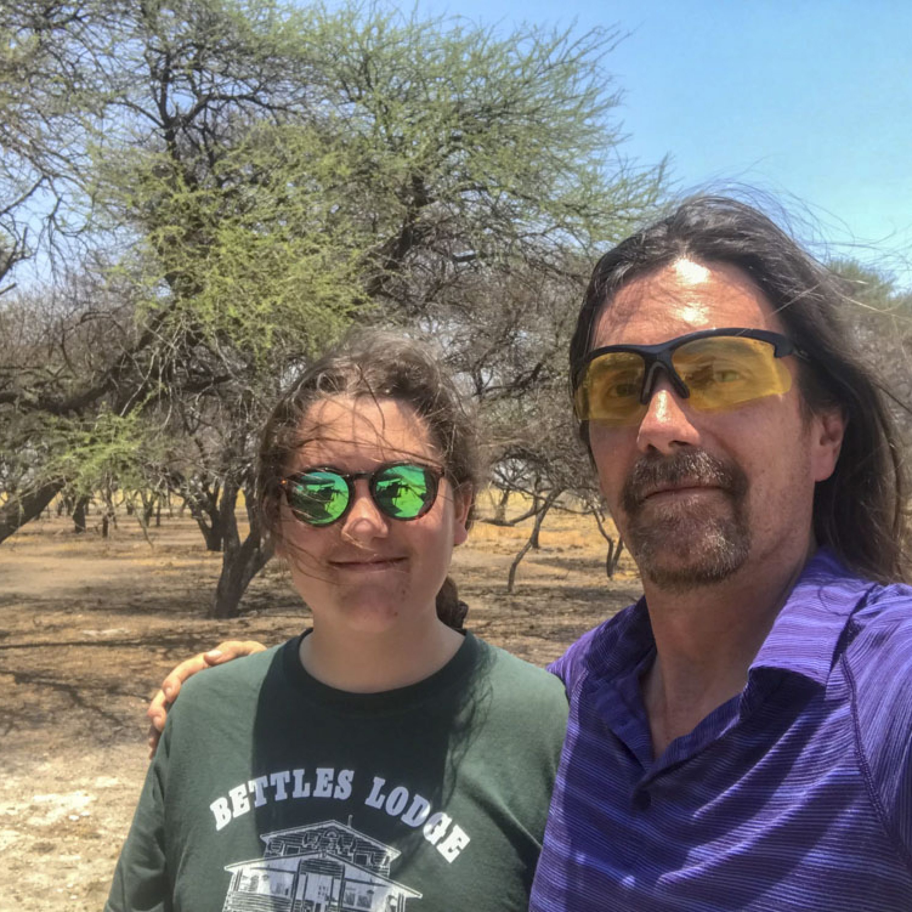
Mopane trees are a favorite food of elephants and cover much of the landscape in northern Botswana. These mopane really want to be enormous, but are stunted at about elephant mouth height. Here’s I am for scale, surveying in a forest of such stunted trees.The first rains were just starting during our November trip, and the leaves were just starting to pop out in many trees. Note how thick the trunks are on some of these shrubs, mopane have adapted to withstand elephant browse and many will continue growing from trunks that have been knocked over by elephants.Here you can see mopane seedlings, stunted trees, and full sized trees. Elephants impact them all. And not just mopane.The Okavango Delta in northern Botswana is truly one of the great wonders of the world, a fascinating mixture of unique geological history, hydrology, and ecology, as is most of Botswana really. There are many good documentaries online, as well as several great books, such as this one.
Our work this year was focused on several transects emanating from or connecting the Linyanti and Okavango swamps. These swamps persist throughout the year, but swell considerably when the floodwaters from Angola arrive starting in early winter there. I had mapped two these transects last year as a demontration, as well as some areas near Maun, so this year we were able to repeat all of those and then some.
Acquisitions
Turner and I arrived in Maun on Saturday November 4th after a several day journey. The major stress in packing was trying to ensure that if any one bag got lost I could build a system with whatever remained. I took the essentials of one complete system with me as carry-on, which was fine except the airlines wanted to limit us to only 8 kg and gave us some grief about the lithium ion batteries, so we had to get creative on check in. But in the end all went well, everything arrived, and before long we were saying hello again to our hosts at the same hotel we stayed at last year.
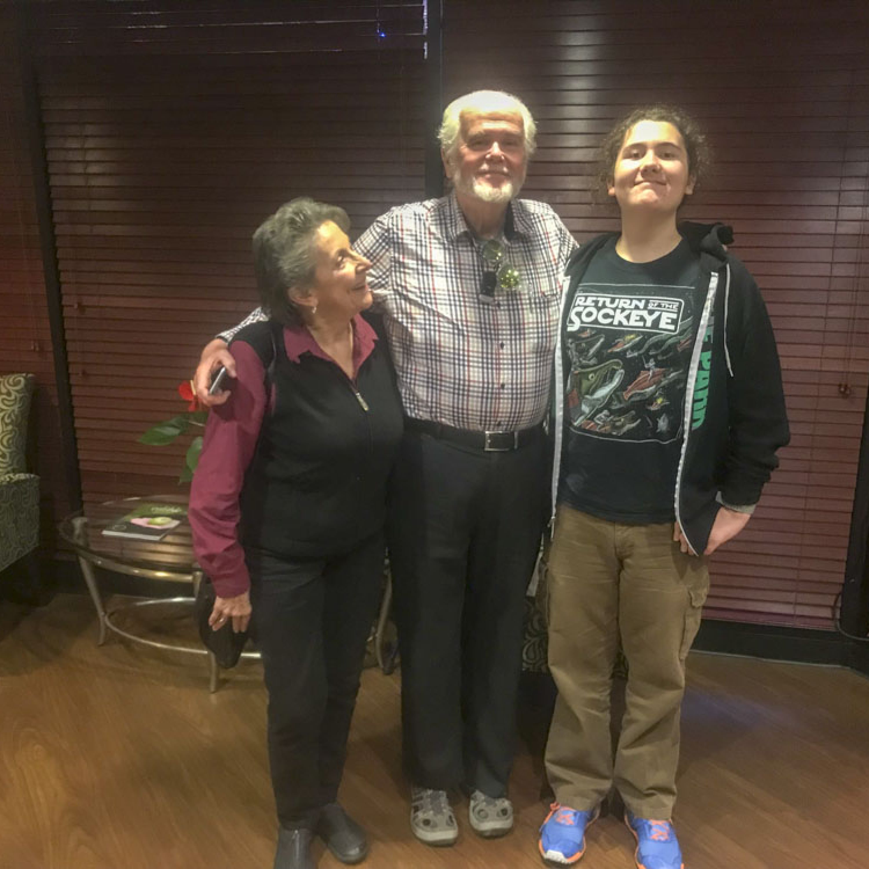
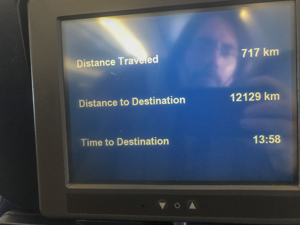
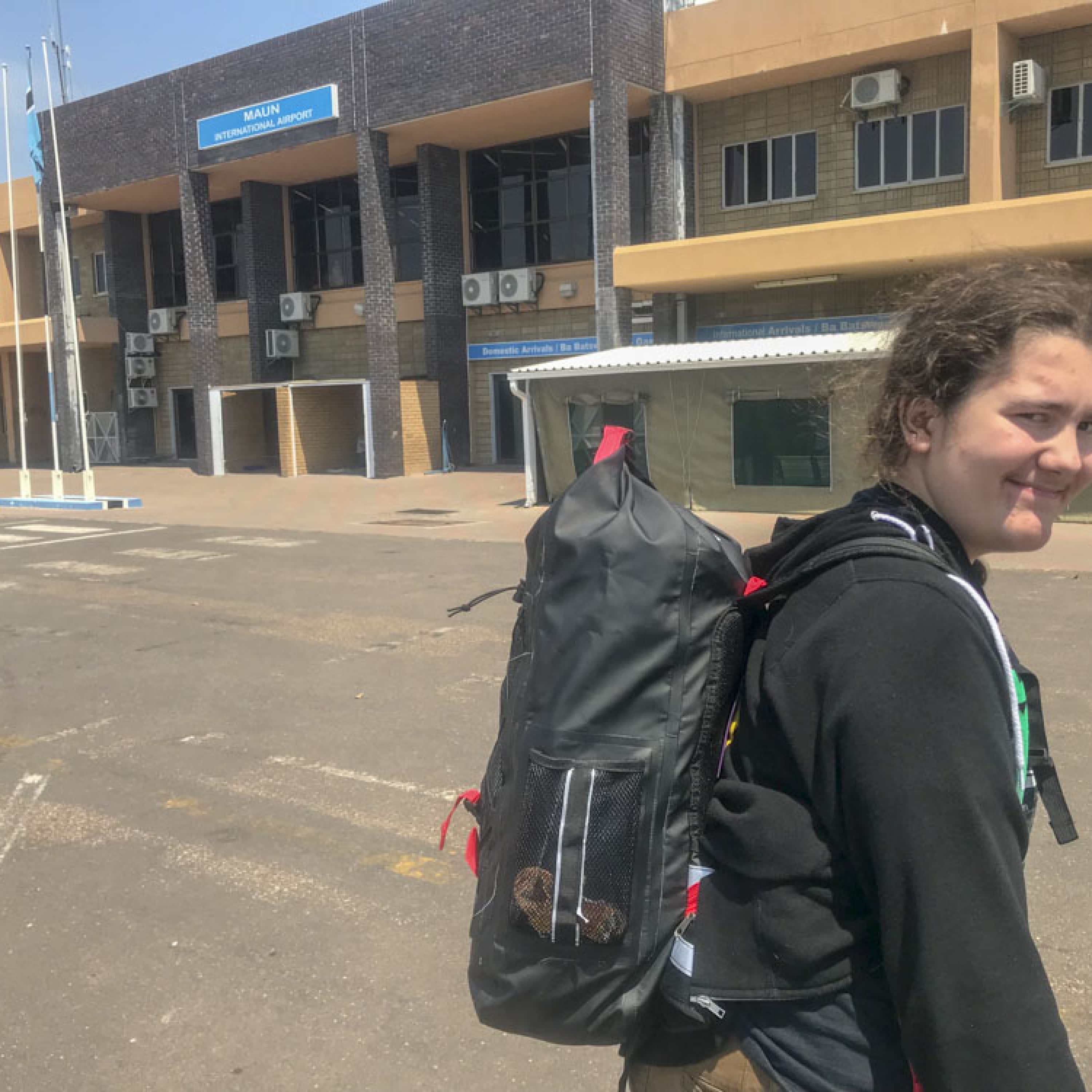
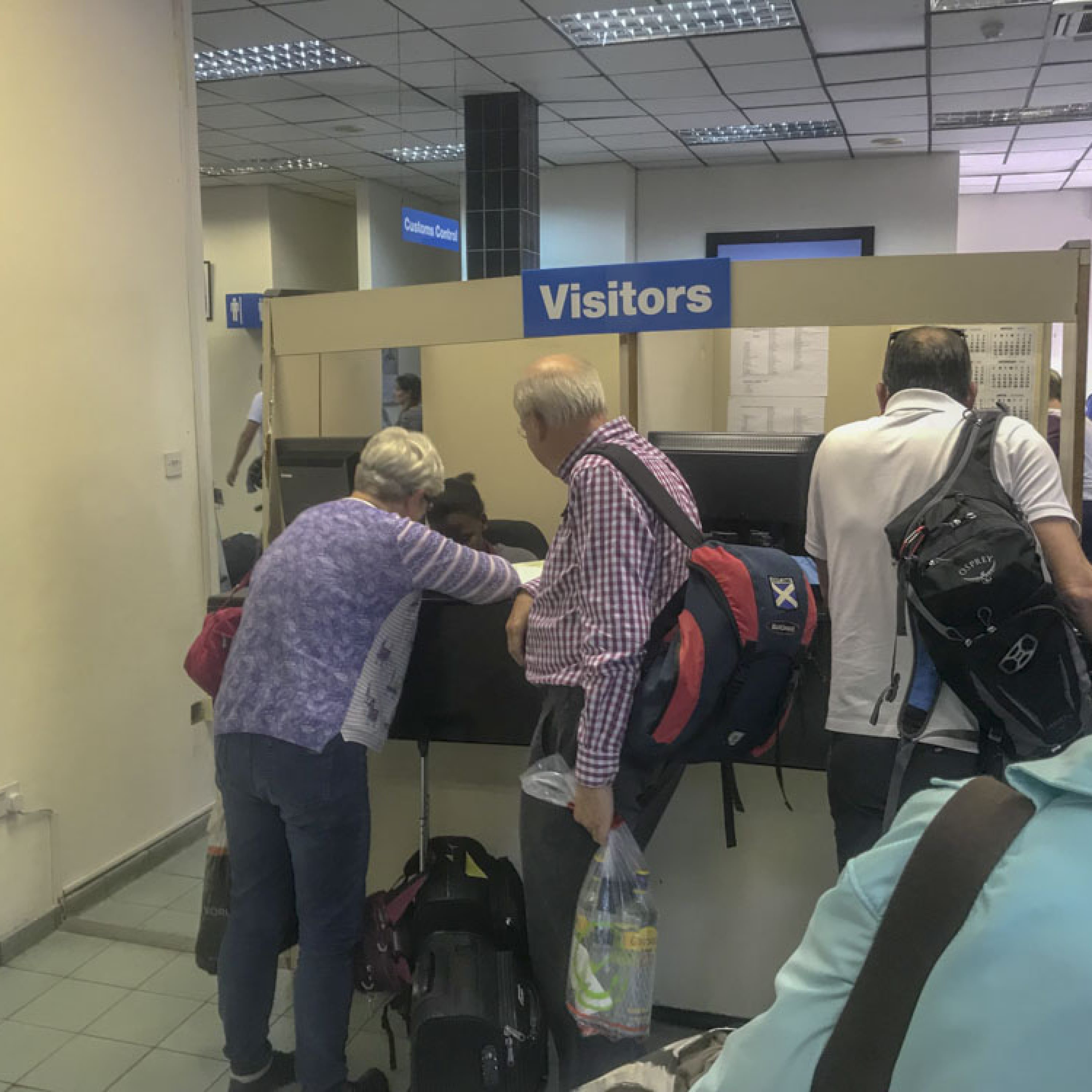
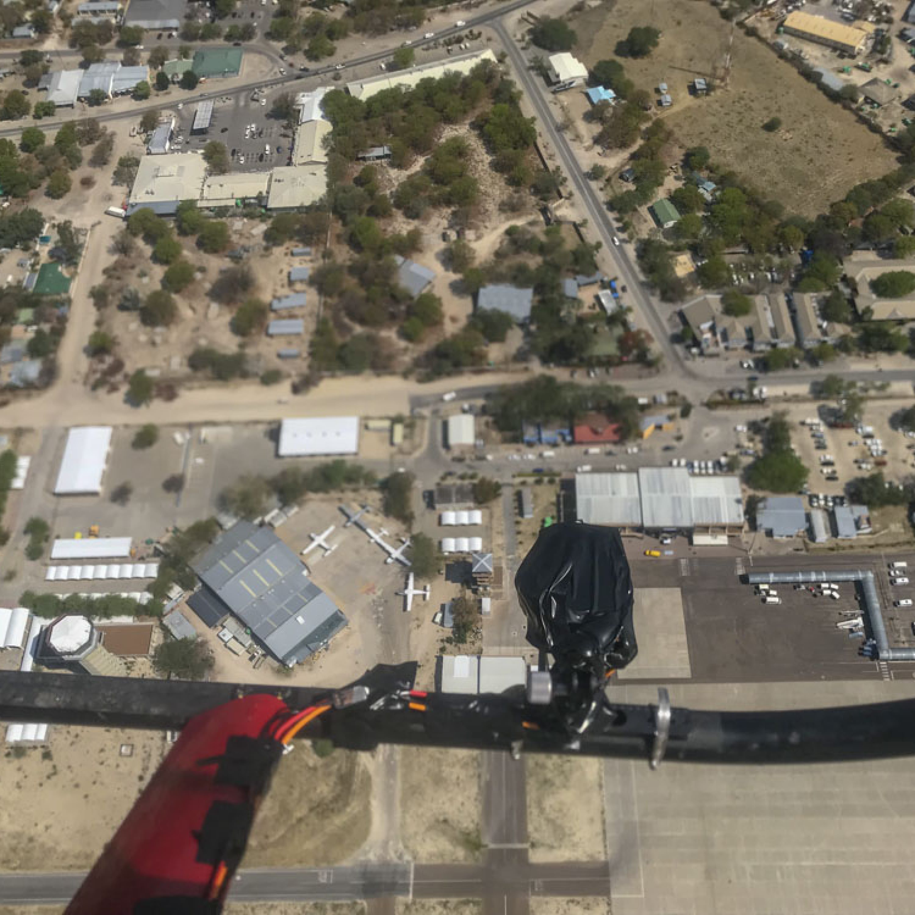
We had a layover in NJ so Turner could pretend to be taller than his grandfather.It’s a long flight from NJ to southern Africa.Maun Airport, finally. I found it interesting how the level of a security changed during our trip, yet I felt safer the less there was.
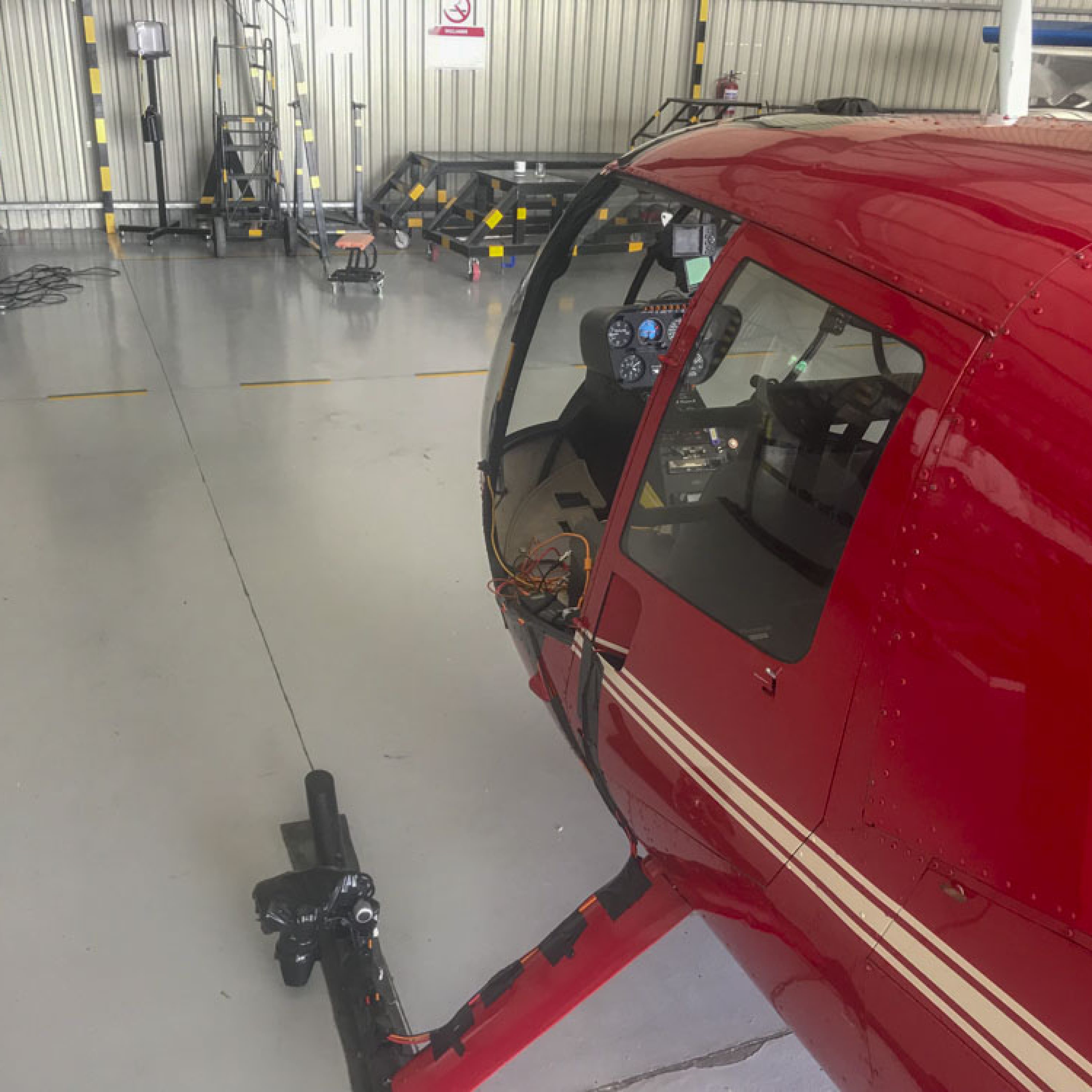
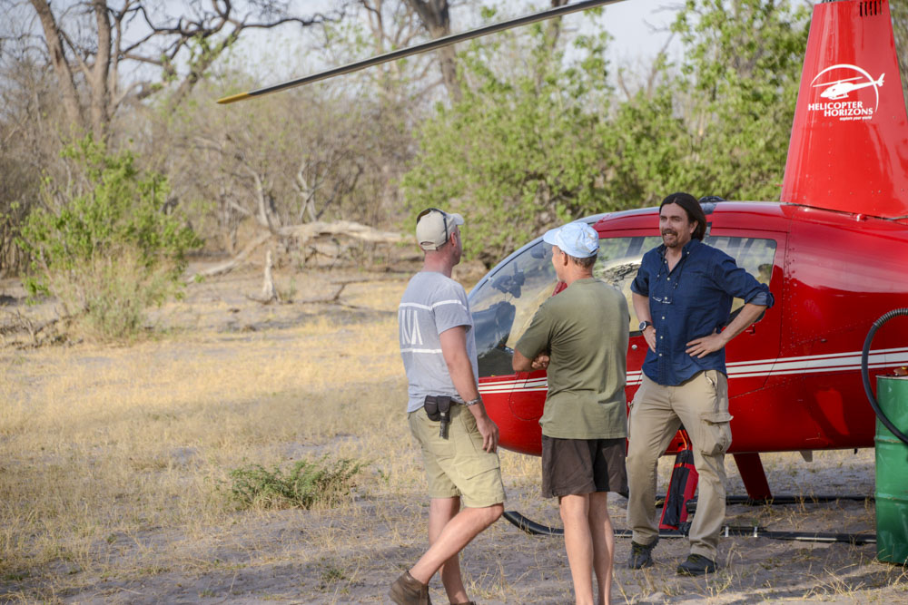
The next morning we were up early to begin our flight testing. It’s one thing for all the gear to arrive, it’s another to make sure it’s still all functional. The owner of Helicopter Horizons, Andrew Baker, picked us up at the hotel and successfully navigated us through the airport security with all of our gear. It is such a pleasure to work with such a great company. Maun is the busiest airport in southern Africa — there are many dozens of caravans, 206s, and airvans parked on the ramp, as well as Andrew’s 10+ R44 and JetRangers, and they seem to all be busy each day. Andrew has been on the scene here for decades and seems to always be excited about something new and useful to do with his helicopters, so despite them being solidly booked he has been at great at finding a way to fit us into their schedule.
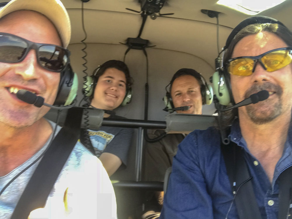
We spent our first full day in Botswana setting up in the hangar, testing the system, and working with our new pilot Joe to learn the ropes of flying in a straight line at a constant altitude rather than hot-dogging for tourists above the wildlife. I’m being a bit glib, but there is a major difference in these flying styles and as a pilot myself I know it’s not easy to master flying straight and level within a wingspan. But it was not long before Joe had mastered it and that night I confirmed everything worked as planned, so we were ready for some real work!
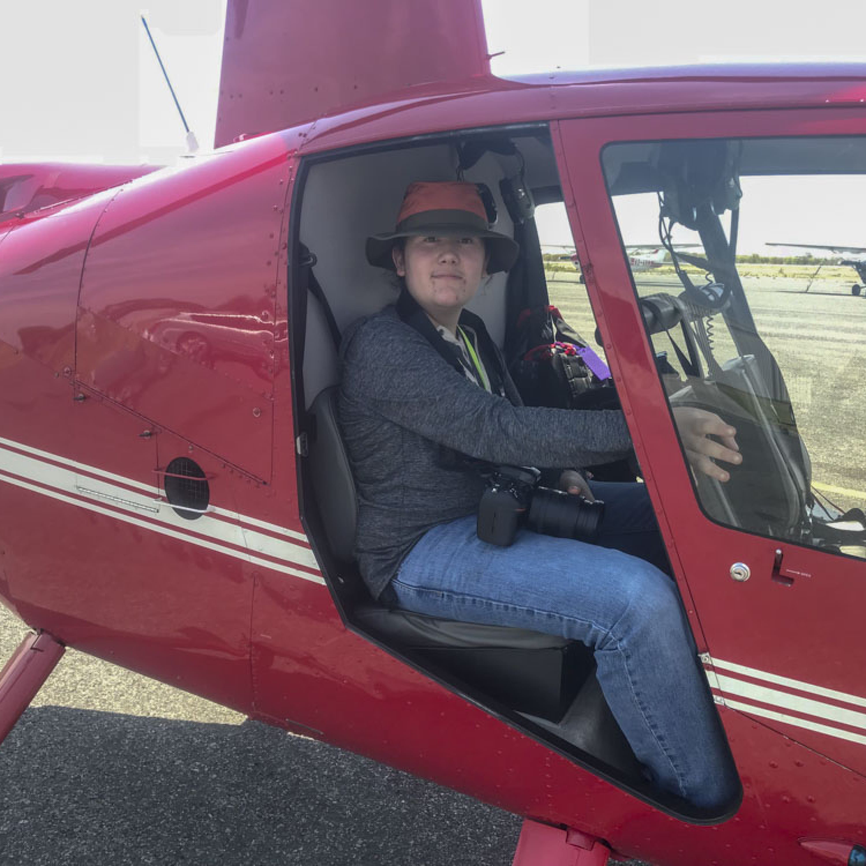
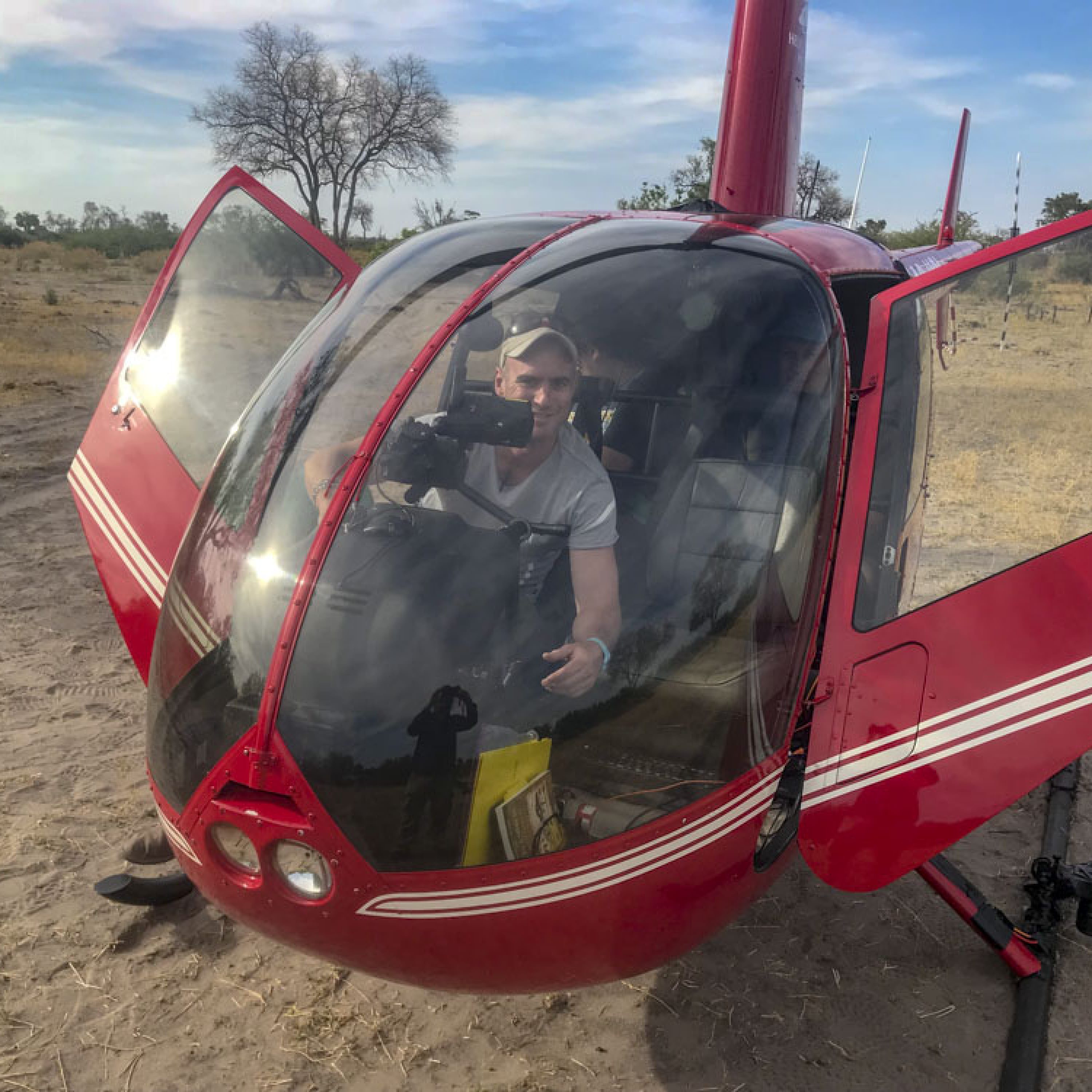
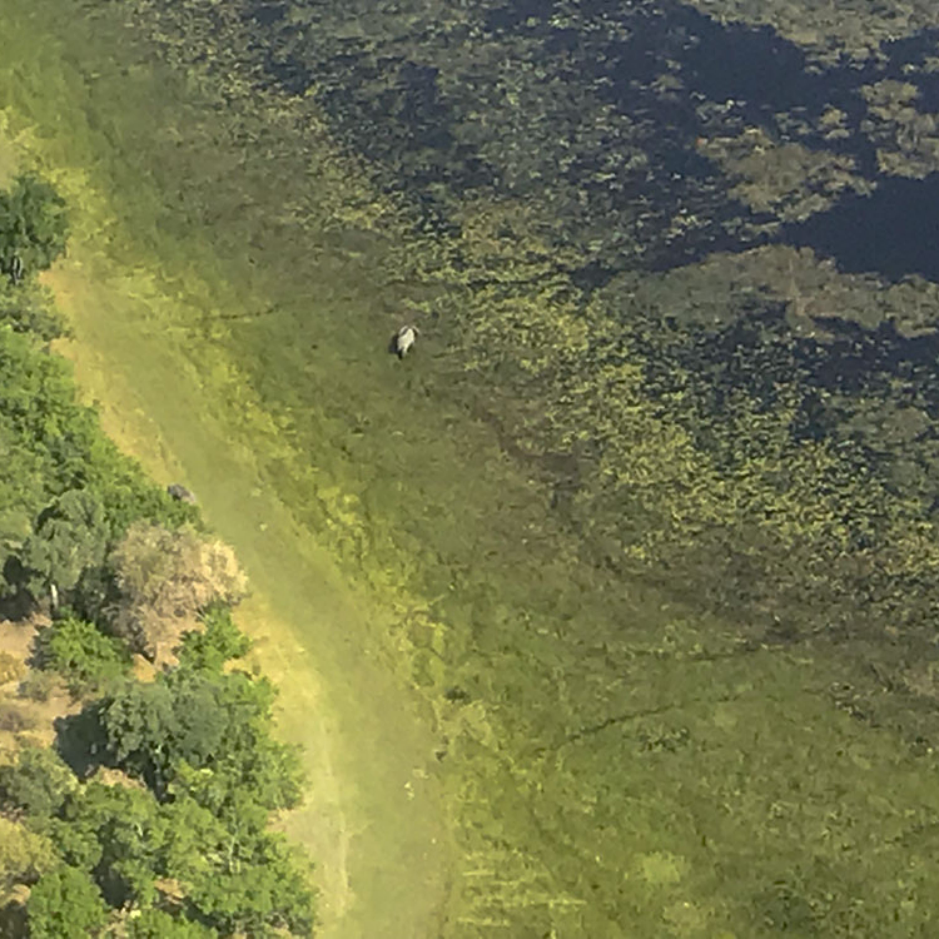
It didn’t take long to install the system. I had hoped to bring a more sophisticated mount this time, but this works well enough and after some testing we were able to improve it further for the real work.Turner is ready to go!We used the airport as a system shakedown, like last year.We also mapped part of the Boro River, like we did last year, as an easy test for change detection methods.A lone elephant enjoys some swamp time.Botswana is really flat, and the difference between swamp and dry ground is measured in decimeters.Would you buy a used map from these guys?In the evening I processed data while Turner brushed up on his ecology.
How that real work was going to occur was still in something of a gray area. Plans were developing rapidly and changing daily even after our arrival, but the general plan was that we would base in the operations camp of the Great Plains conservation company near Selinda, dubbed CSU camp, as it was central to most of our transects and would greatly reduce commute time. Great Plains appears to be one of the most active and progressive conservation groups in Botswana and southern Africa, in addition to running a series of top of the line safari lodging sites. So we spent the first half of the day at the Okavango Research Institute with the lead scientist of the project Dr Richard Fynn, giving a talk and meeting folks, then spent the second half of the day dealing with logistics like buying camp food, organizing vehicles, sorting and packing, etc. The general idea was that Turner and I would fly to CSU with Joe in the R44 while Richard and his wife made the 8-12 hour treacherous drive in a University vehicle, and we should meet up there about noon.
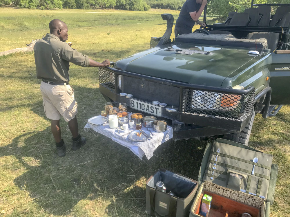
Shopping for food for a week of field work.
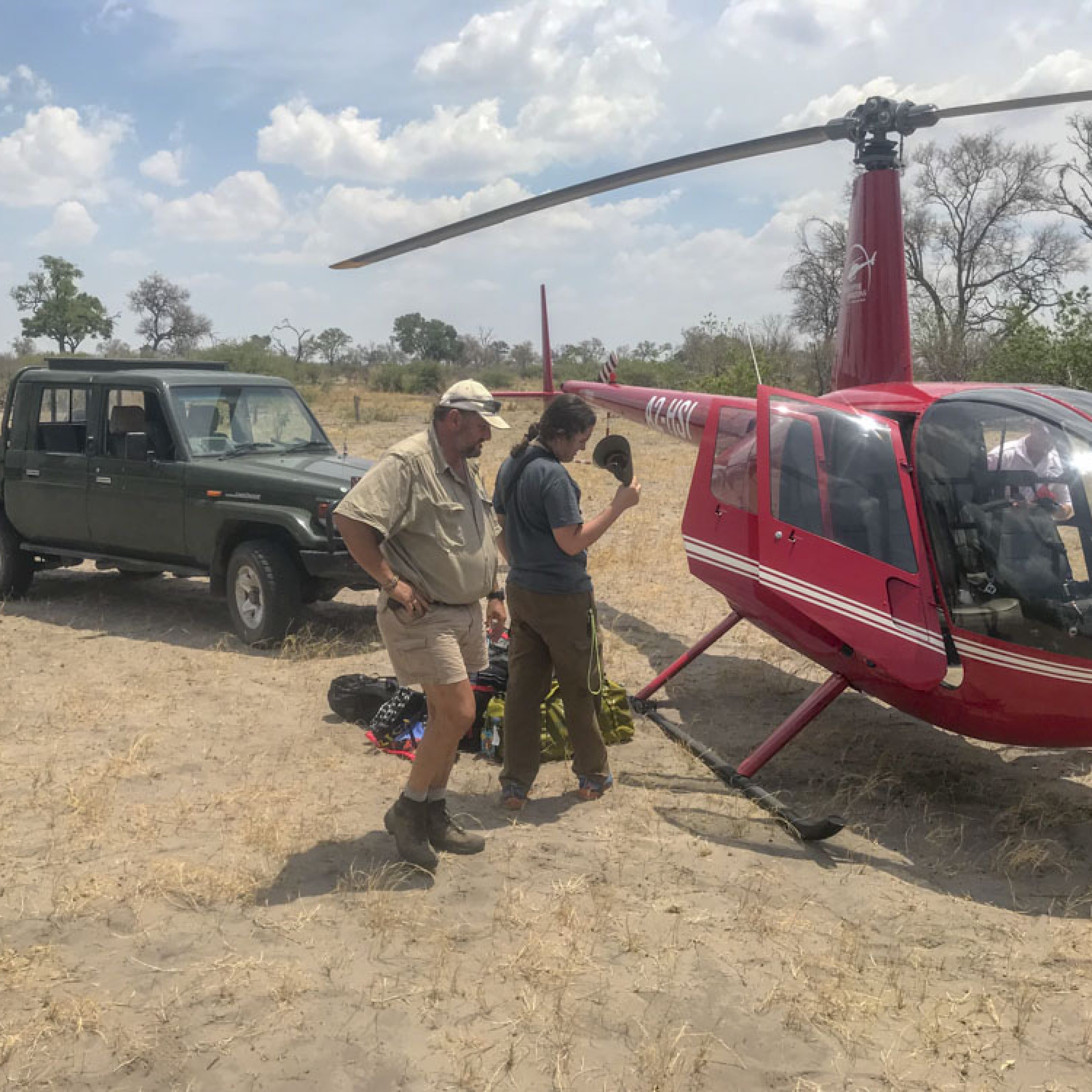
That plan worked out reasonably well. Turner and I met up with Joe early in the morning, rigged and tested the system, smushed all of our other gear inside, flew about an hour over the scenic landscape, tossed out the gear into a waiting truck, reorganized a bit, and were mapping by about 9AM. Partly by design, partly by luck, each of our mapping blocks was just about the ideal size and distance to complete comfortably on one tank of gas. By the time returned from our first block, Richard and Theresa had arrived, and Richard joined us for the second block. So basically within 72 hours of arrival we had almost a third of work complete!
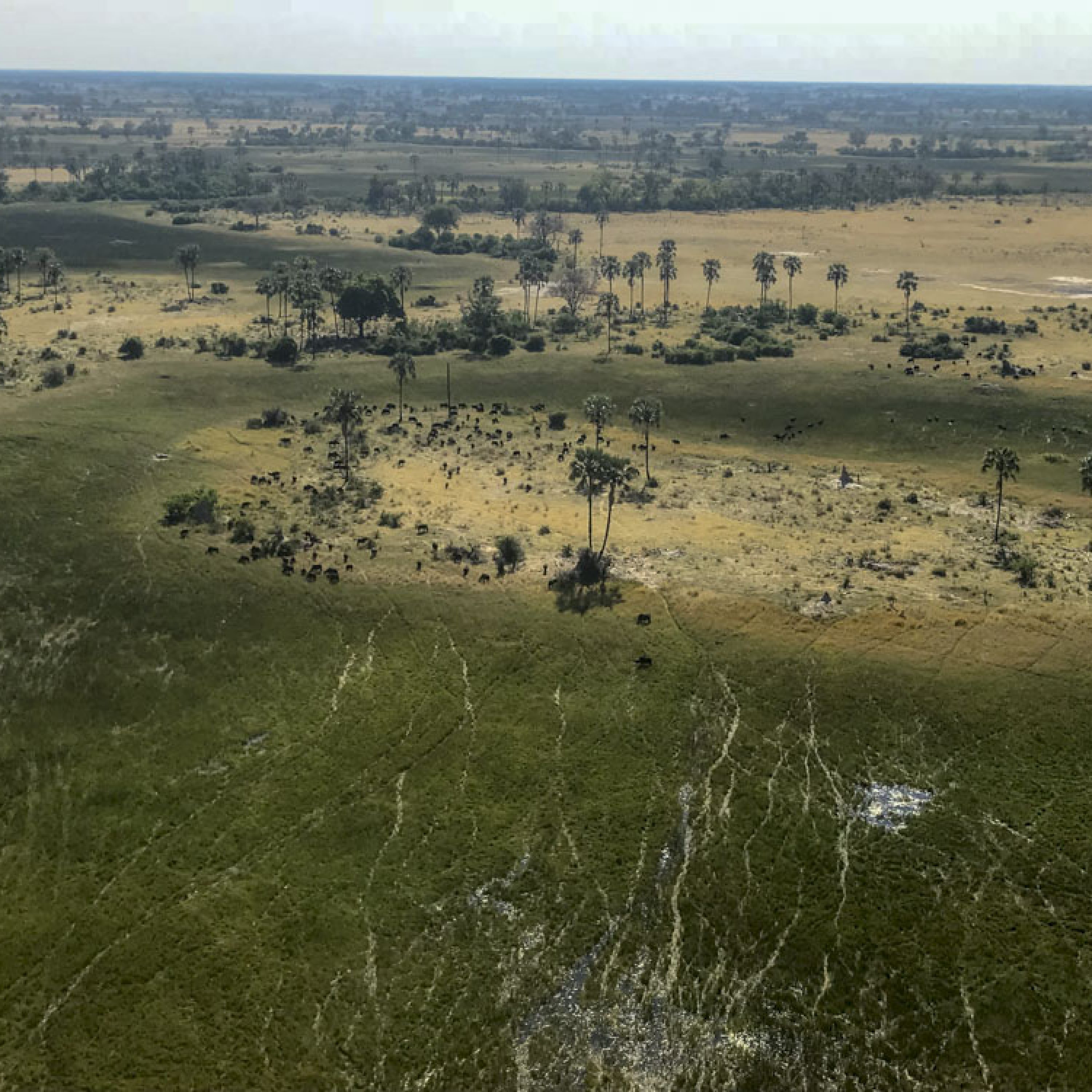
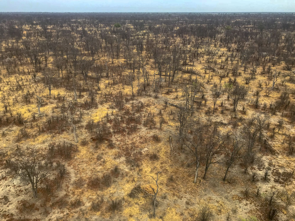
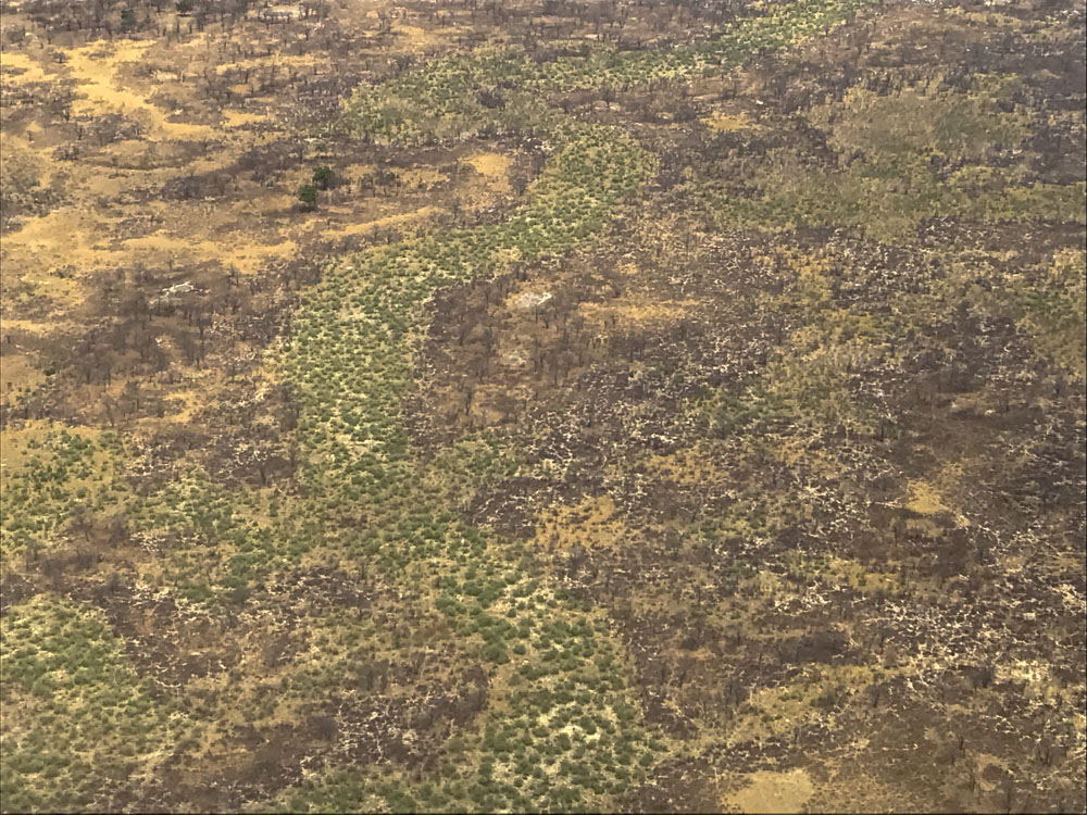
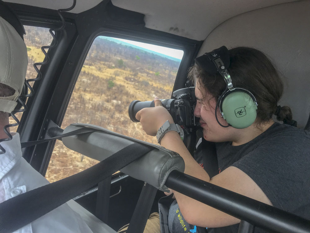
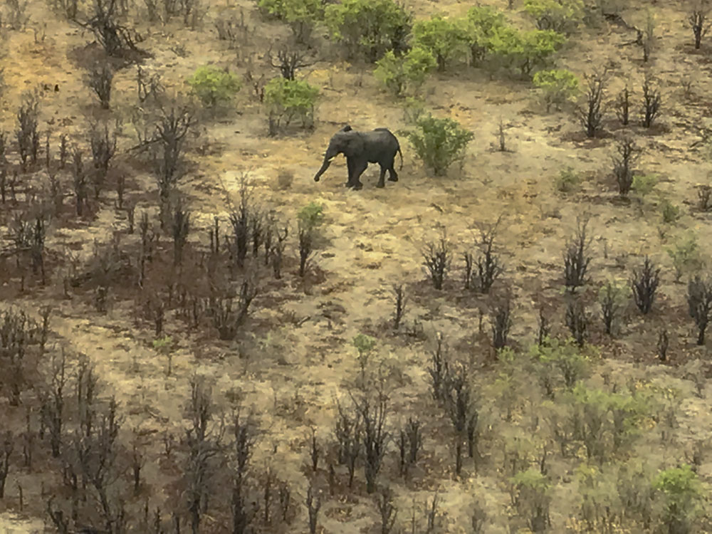
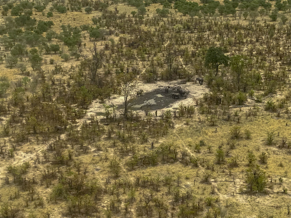
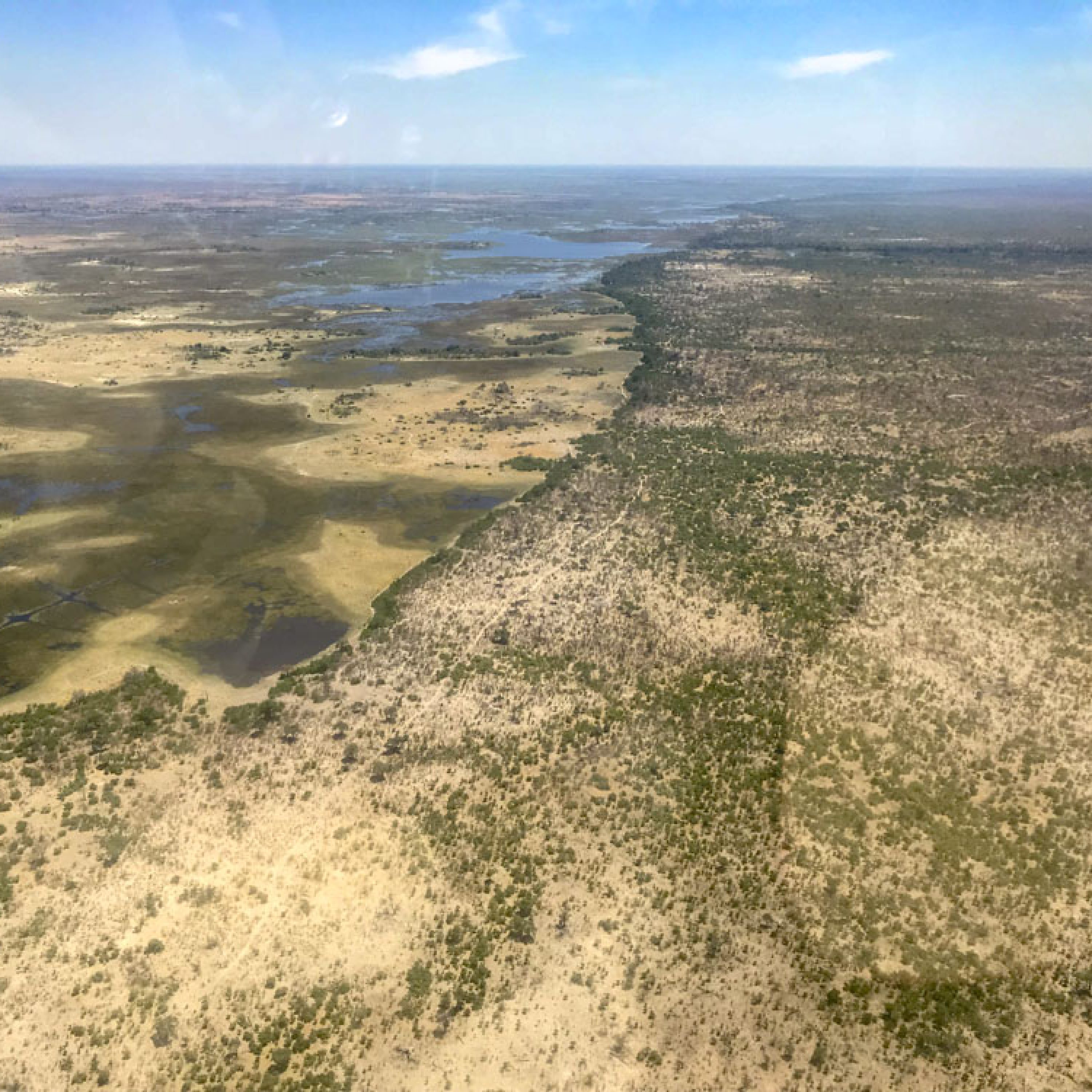
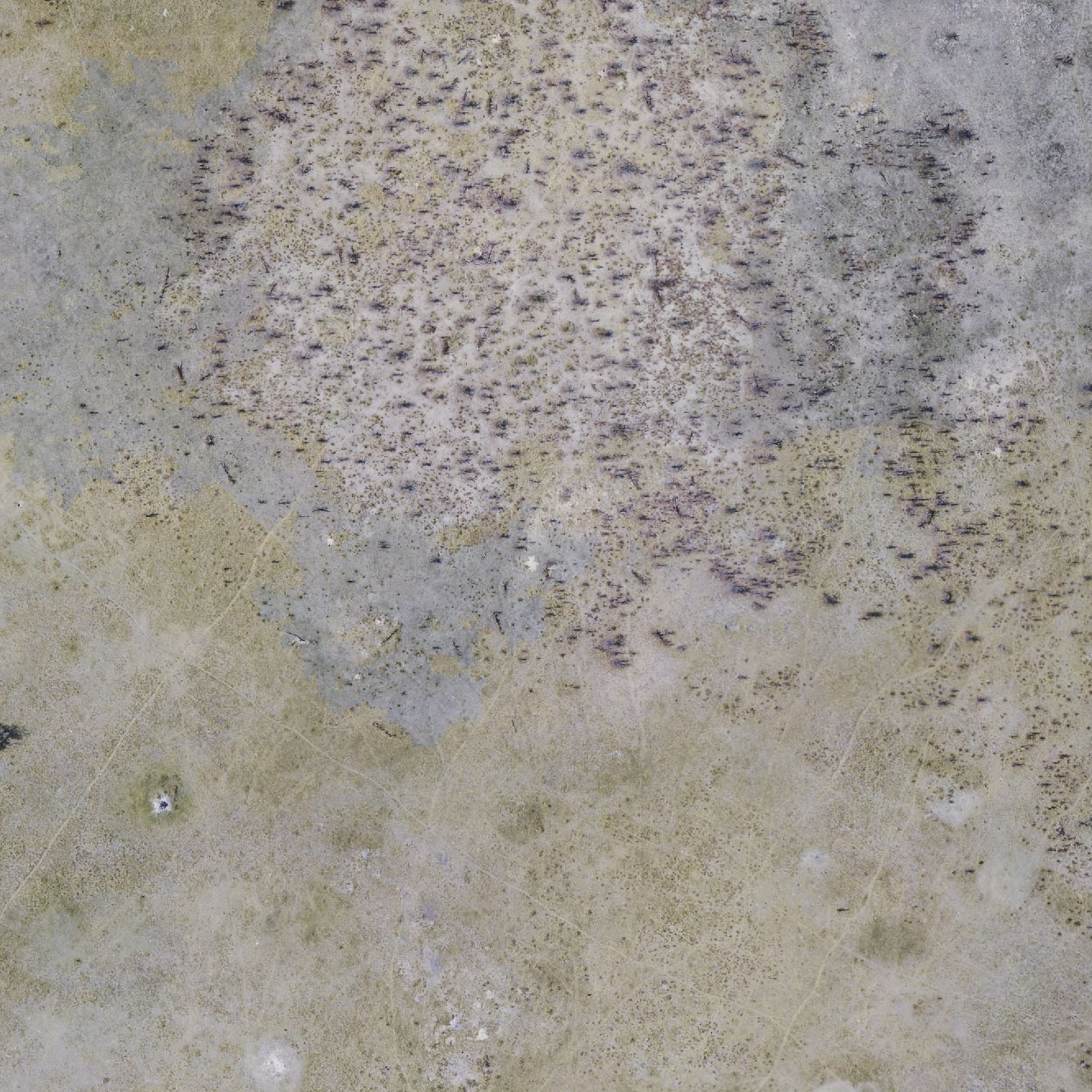
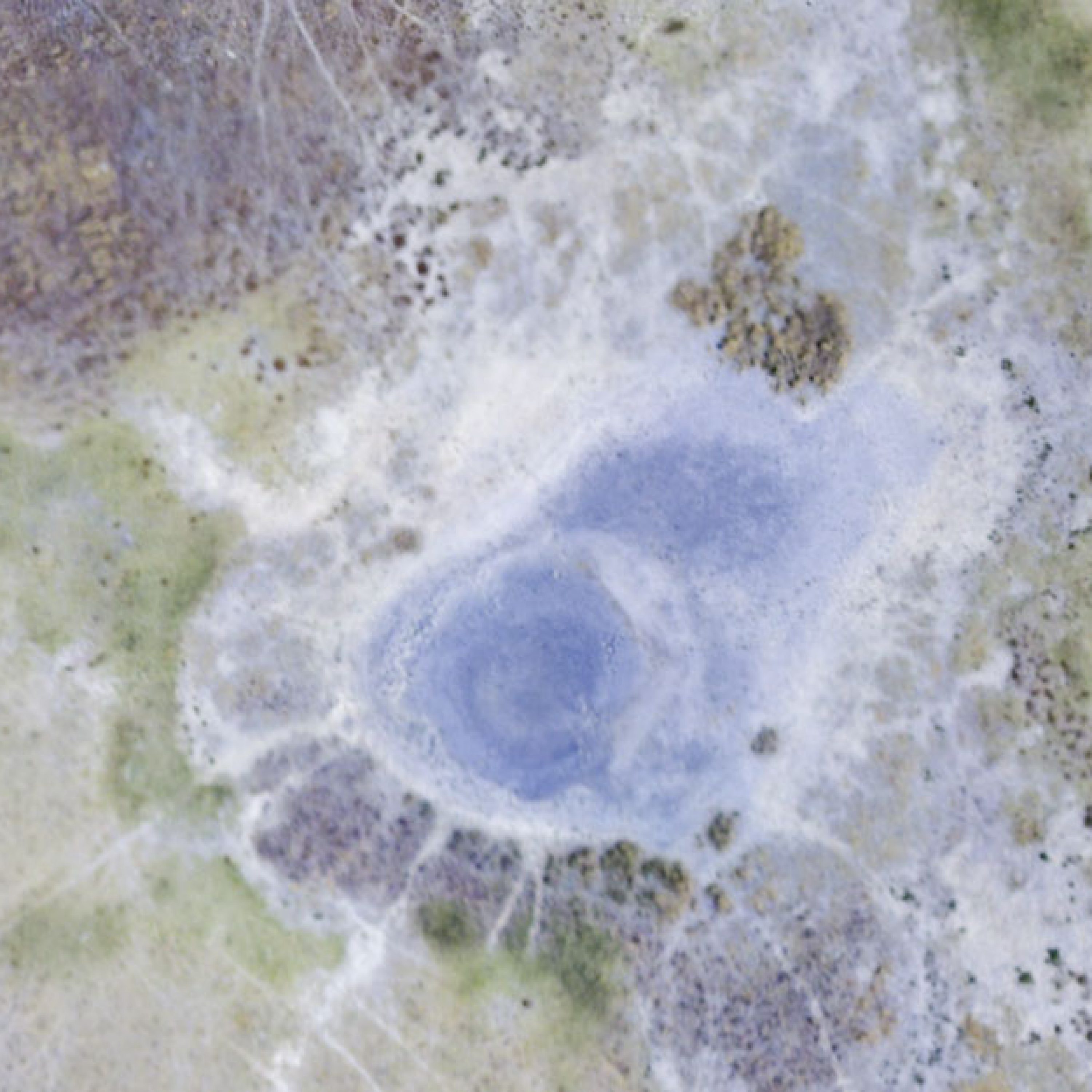
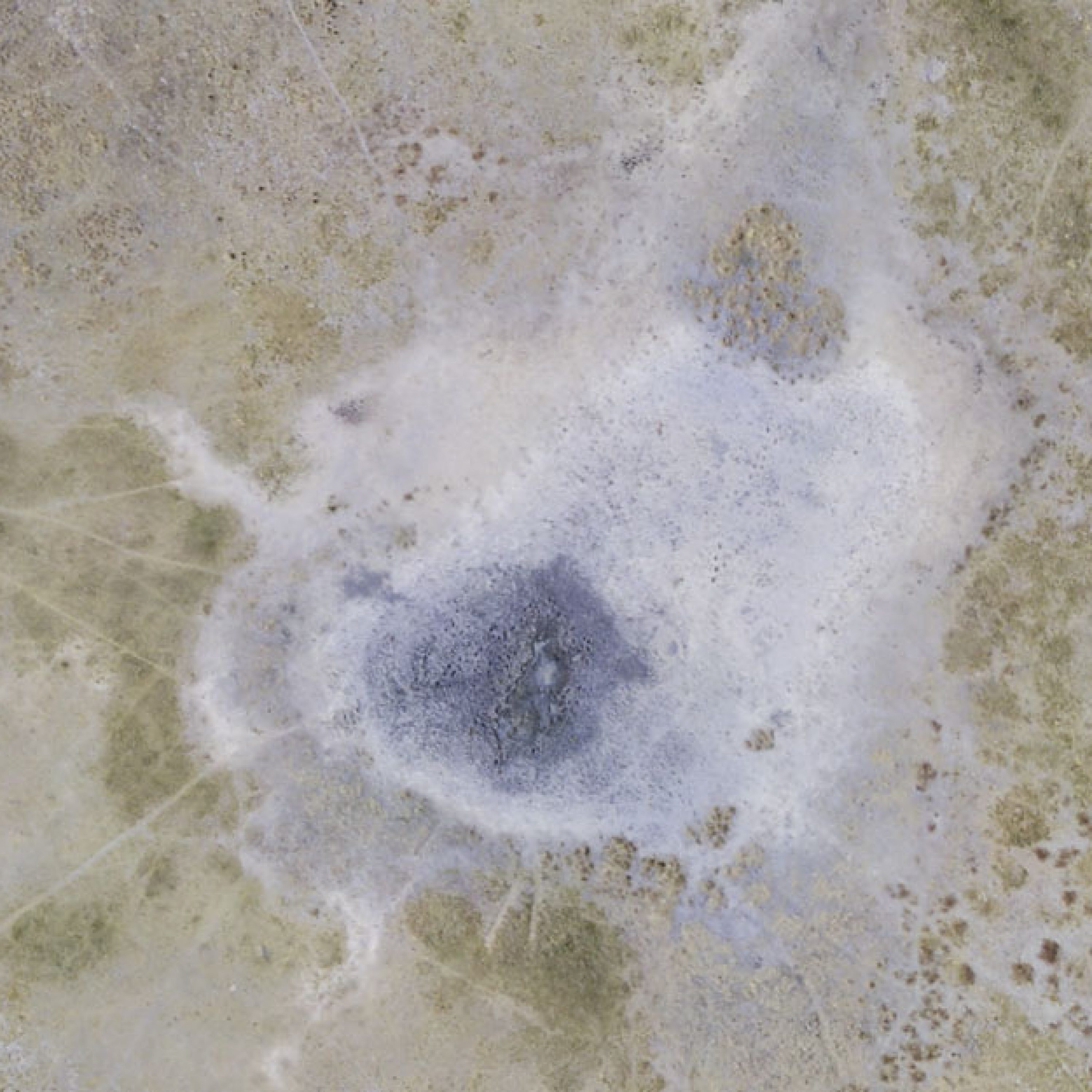
The landscape in northern Botswana is heterogeneous, with subtle variations in topography exerting a strong control over the ecology.The landscape largely controls the hydrology, which in turns largely controls distribution of vegetation, which in turns largely controls the distribution of wildlife. In the case of elephants, their use of permanent water bodies created by the landscape and hydrology creates impacts on woody vegetation that decrease with distance from those water bodies, exerting another control on ecology. Or at least that’s what we would like to test.Botswana is in a unique geolocatical setting, with subtle shifts in plate tectonics causing large changes in hydrological dynamics due to how flat the landscape is. Much of northern Botswana is covered by these fossil river channels, that apparently became choked with sand as they dried up due to drainage changes. That sand supports a particular vegetation community, in this case primarily composed of silver terminalia, apple leaf, and shepard’s tree. At the start of the rainy season like here, these trees sprout leaves earlier than the surroundings, making the channels pop out. Of course the leaf-eaters are excited about this too.Just outside the fossil channels the soils have more clay. The dominant woody vegetation here is mopane. You can distinguish them clearly from a distance because the leaf litter from the previous year turns the ground reddish.These channels come in all shapes and sizes. Using the DEMs I created, last year I found that they can be higher or lower than the surround soils, there seemed to be no consistent pattern.Turner found many opportunities to advance his photography skills. You can read his blog of his experience here.Here an elephant browses in a forest of stunted mopane trees, some of which have leaf out already. Notice the trees are cropped just at about elephant mouth height, but would grow much taller otherwise.The lack of mopane leaves where the elephants walk makes their trails stand out and make it obvious that they spend a lot of time in these woods, and anywhere they spend time they eat.Elephants can only go a few days without water, especially the young ones. So the impact of browse as a function of distance from water sources is something we hope to study with these data.The landscape is covered with these small pans. I think they are actually created by the elephants themselves, as they are constantly digging and expanding little holes. Whether they realize that these small holes will eventually become watering holes or if they plan such locations to fill in geographical gaps in water sources, I really don’t know. But I would not put it past them, they are very smart.
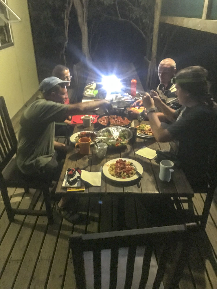
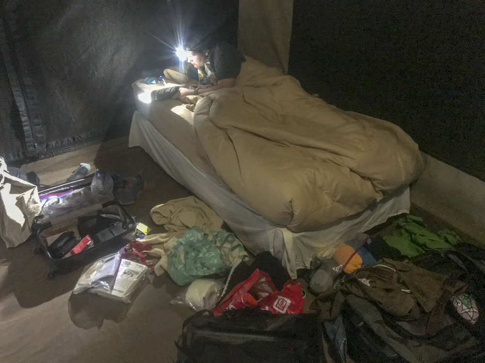
The next two days were a blur of similar activity. I was up before dawn getting the day’s missions organized and up late into the night processing data to ensure what we collected worked as well as we hoped. Turner and I just snacked for breakfast and lunch, and usually in the evenings we ate together if not too exhausted from the work, jet lag, and heat. The lack of internet and power in the late evening made work challenging, but in the end fortunately there were no major issues to deal with and all worked out fine. We even finished a day earlier than planned!
It was a short but pretty walk from camp to where we parked the helicopter.Joe was always ready to go flying.“Rocks, paper, scissors for who’s pilot today…”
Turner takes his turn pumping fuel into the helicopter.
The tip of the Linyanti swamp is defined by a slight rise in topography.Swamp grasses are another favorite food source for elephants, and even here they have some affect on the landscape as their trails influence drainage patterns.We surrounded the helicopter with acacia thorns each night to keep the baboons from opening the doors and wreaking havoc.The mapping crew.
On our final day based out of CSU camp, we did some bootleg ground control by reconfiguring the airborne system into one of the safari vehicles. This worked out great. And soon enough we were back in Maun, scrambling to transition into our next adventures in Botswana.
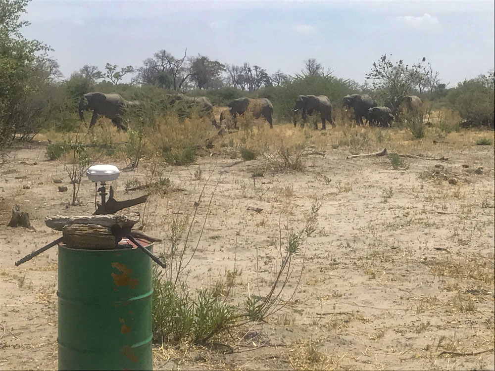
When we arrived John suggested we place the GPS base station on a barrel, as elephants apparently don’t like barrels. Turned out to be great advice!
And apparently giraffes don’t like landing helicopters…
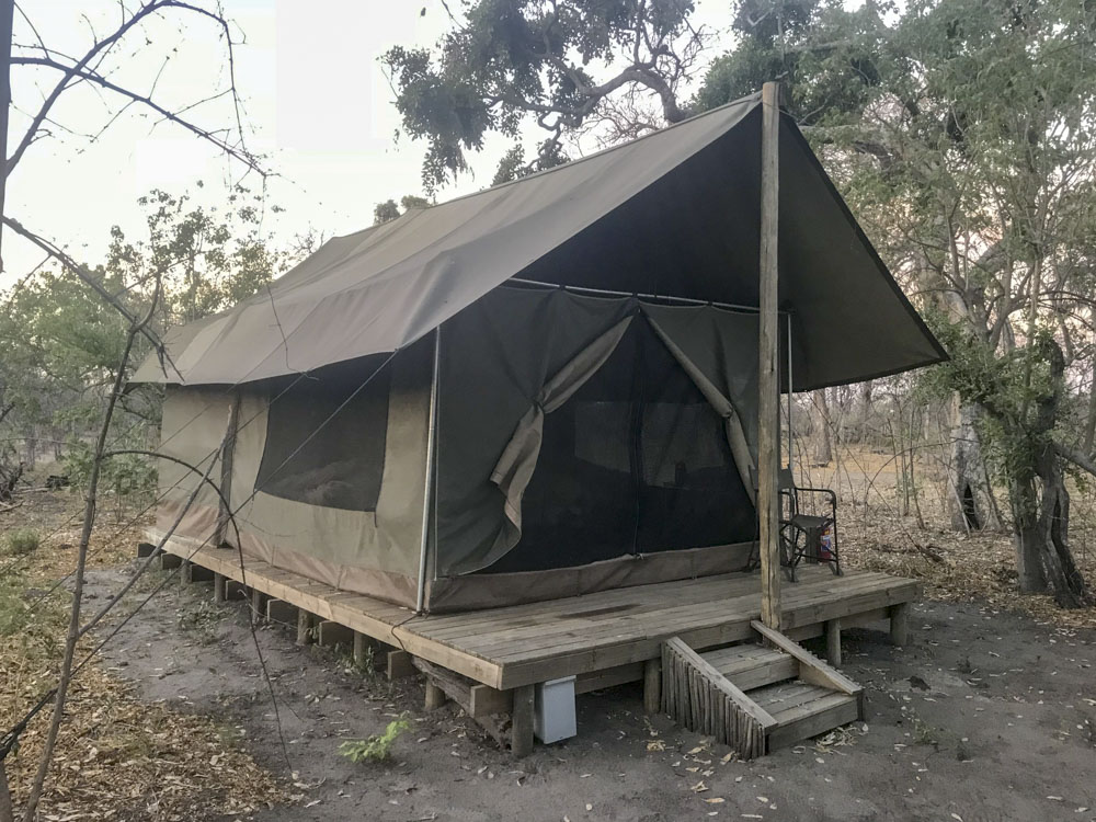
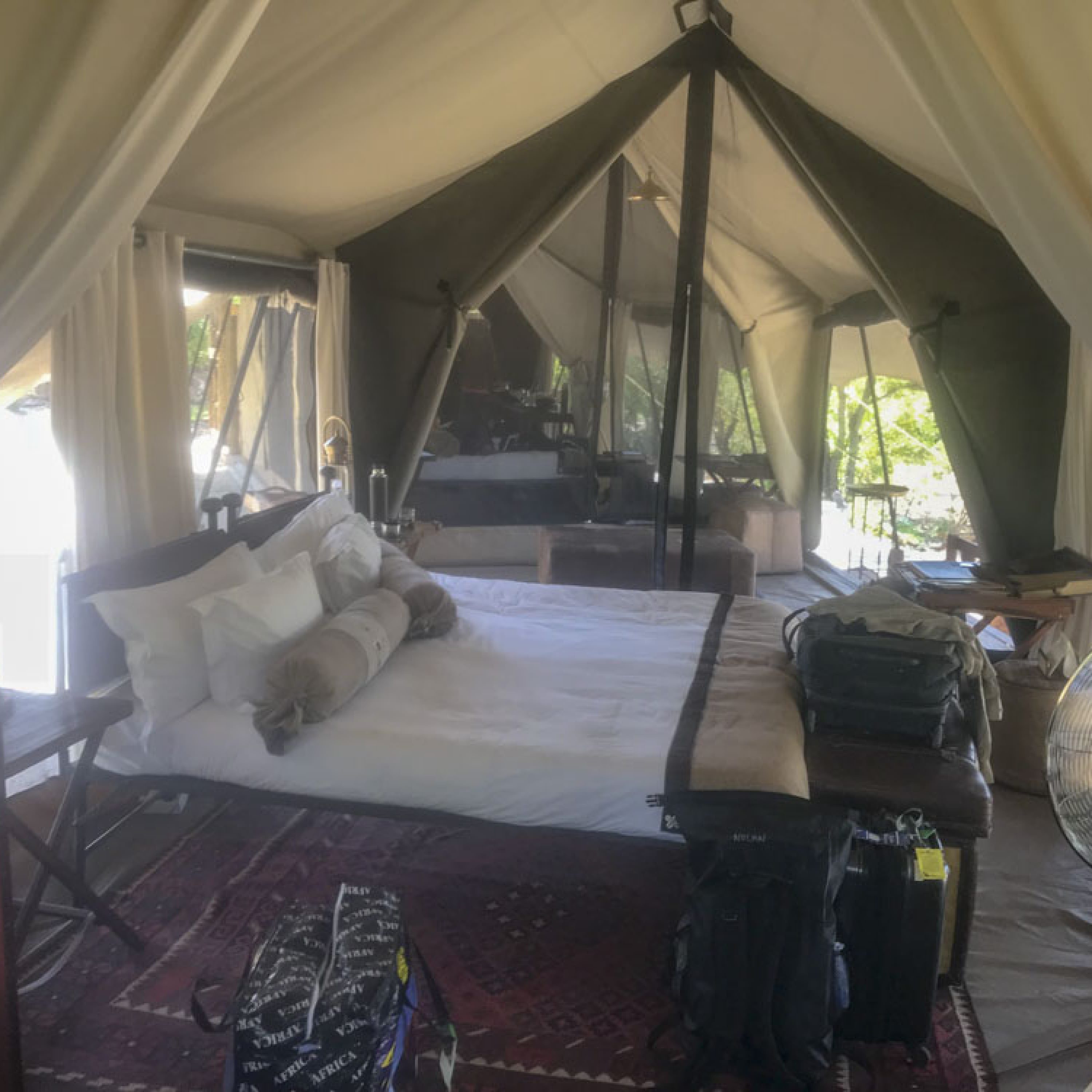
Dinners happened late at night after long days of work.Our home away from home at CSU camp. Compared to Alaskan field work it was deluxe.Our tent had beds with sheets and a bathroom!Stuffing the helicopter full on our way back to Maun.
My general idea in planning this trip was spending the first week or so doing the airborne mapping and the next two weeks learning ecology on the ground and doing some field work based out of safari lodges in or near our study areas, with one week open at the end of the trip. In this way, if any of our system gear got lost or stolen or broken or the logistics fell through in some way, we’d have roughly two weeks to sort that out and could try again at the end of the trip. Fortunately that wasn’t necessary, so we were able to get a lot more learning experiences in on the ground over the next three weeks, as well as becoming increasingly sophisticated with our ground control methods using a safari vehicle. The rest of this blog discusses the data itself, how we validated it, and some sample analyses.
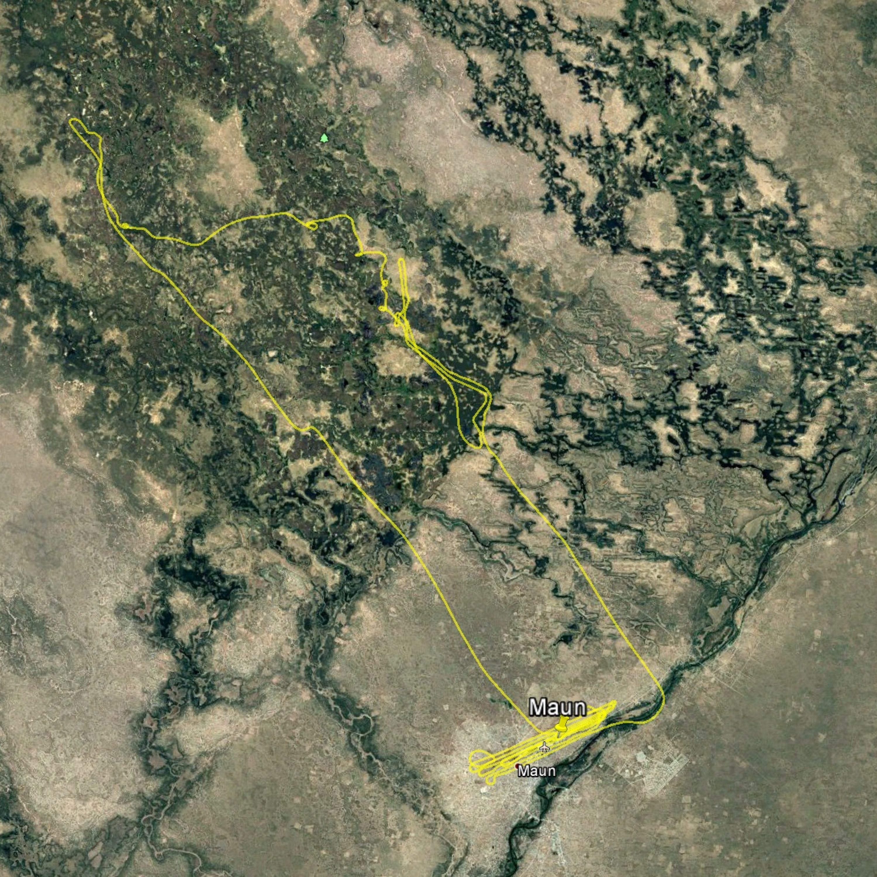
On our first fully day in Botswana, 4 Nov 18, we mapped the airport in Maun and a stretch of the Boro river as shakedowns. We had mapped both these areas in 2017, using these areas as local validation testing sites of urban and wild terrain.
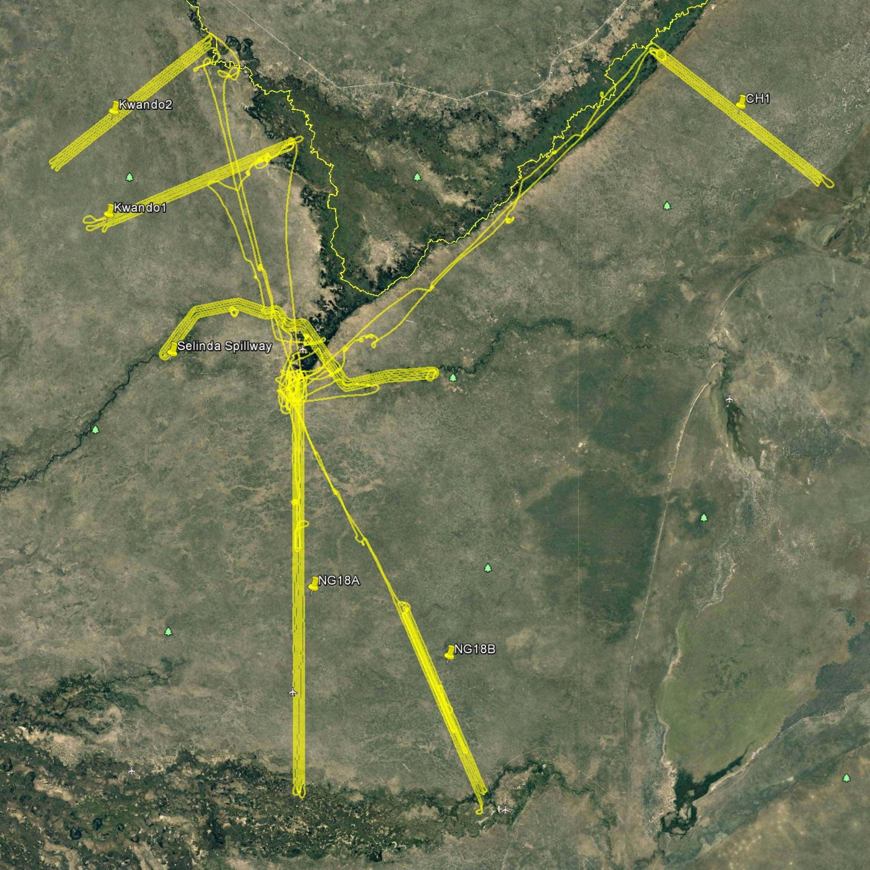
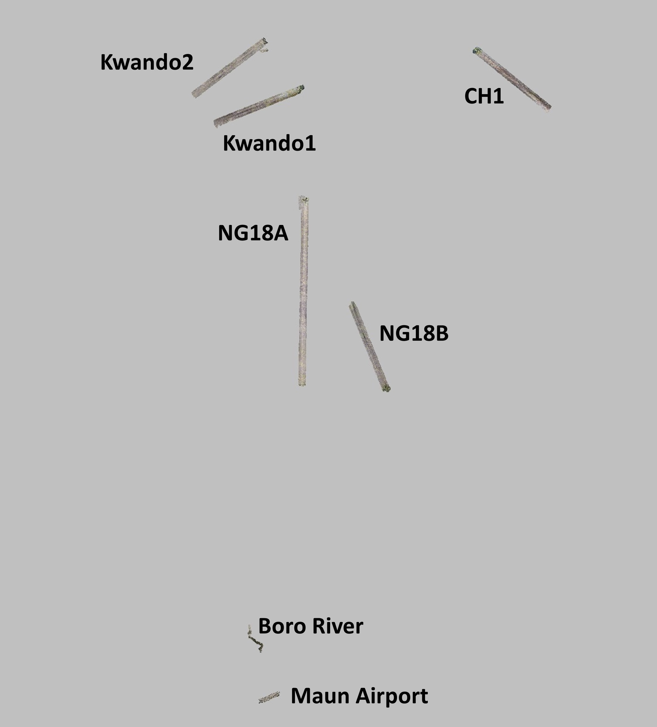
Here are our flight lines while based at CSU camp (just left of center at the top of NG18A where all the flight lines converge).
The Data
We mapped Kwando1 and CH1 first (6 Nov 18), Kwando2 and NG18A next (7 Nov 18), and NG18B and the Selinda Spillway (not shown here) on our last day of mapping there (8 Nov 18). We returned back to Maun the next day, after doing some ground control in NG18A and the Spillway blocks. The shorter blocks are about 25 km x 2 km, and NG18 is 50 km long.
All of the transect data shared the same specifications: – Photos were acquired at 10 cm GSD and orthomosaics posted at 10 cm – Point clouds had an average point density of ~25 points per meters squared – Digital Elevation Models were posted at 20 cm – Precision/repeatability is ~15 cm – Geolocational accuracy is ~1-2 pixels horizontally and ~30 cm vertically (though see validation notes below regarding vertical) without ground control – No ground control was used in processing these airborne data, only in validating it – Data delivered in WGS84 UTM34S, no geoid model applied.
In this section I try to give some flavor of the data, including a top view of the orthoimage and DEM for each block as well as a video or two flying over the point cloud. They don’t really do the data justice, but internet sharing tools for these type of data just haven’t caught up to the acquisition technology yet so best I can do in the meantime.
Kwando1 Block
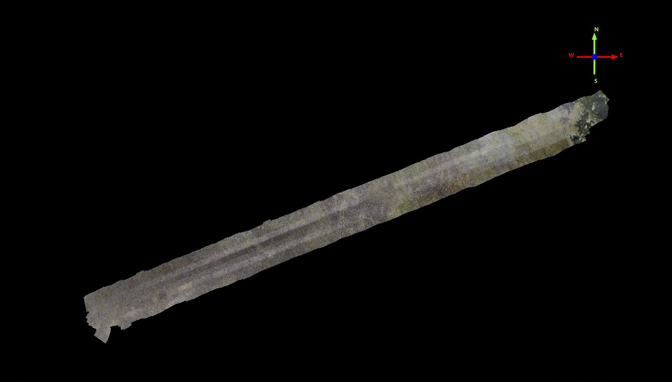
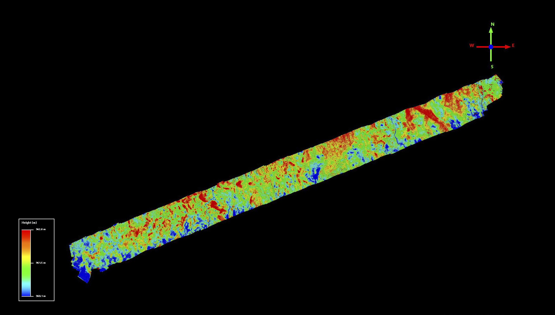
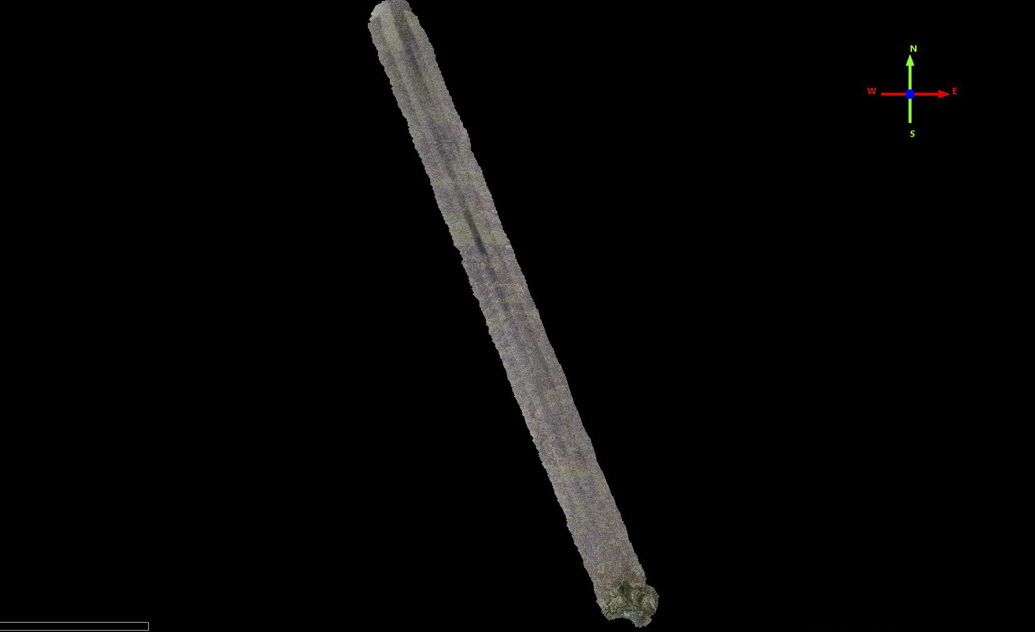
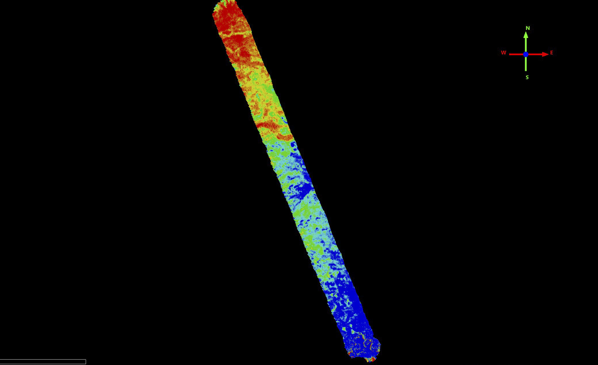
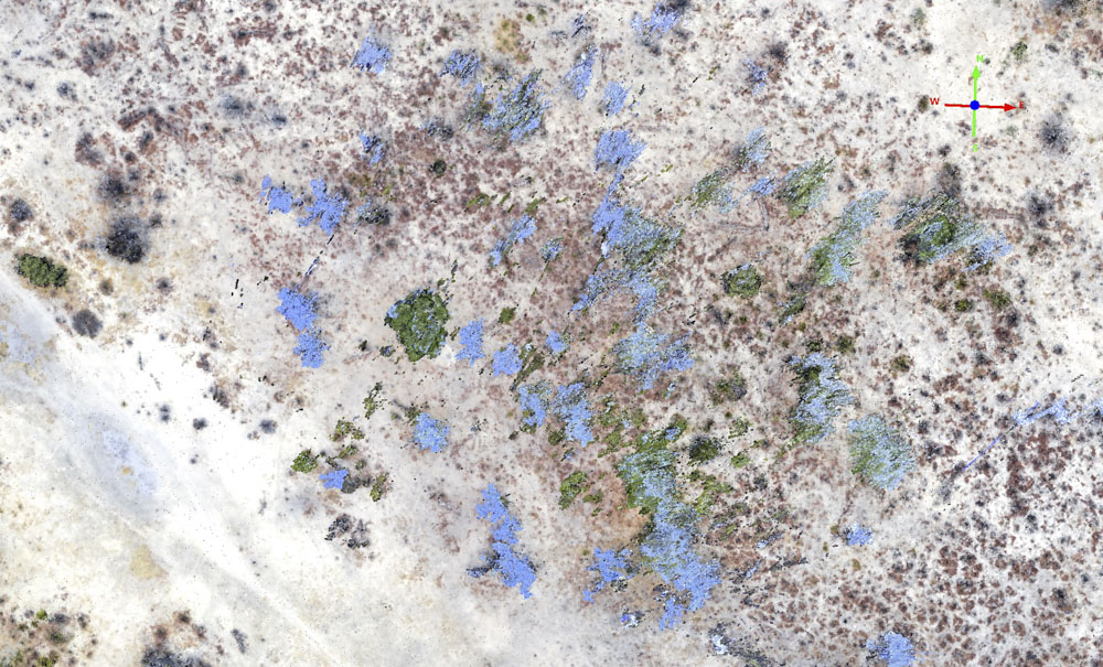
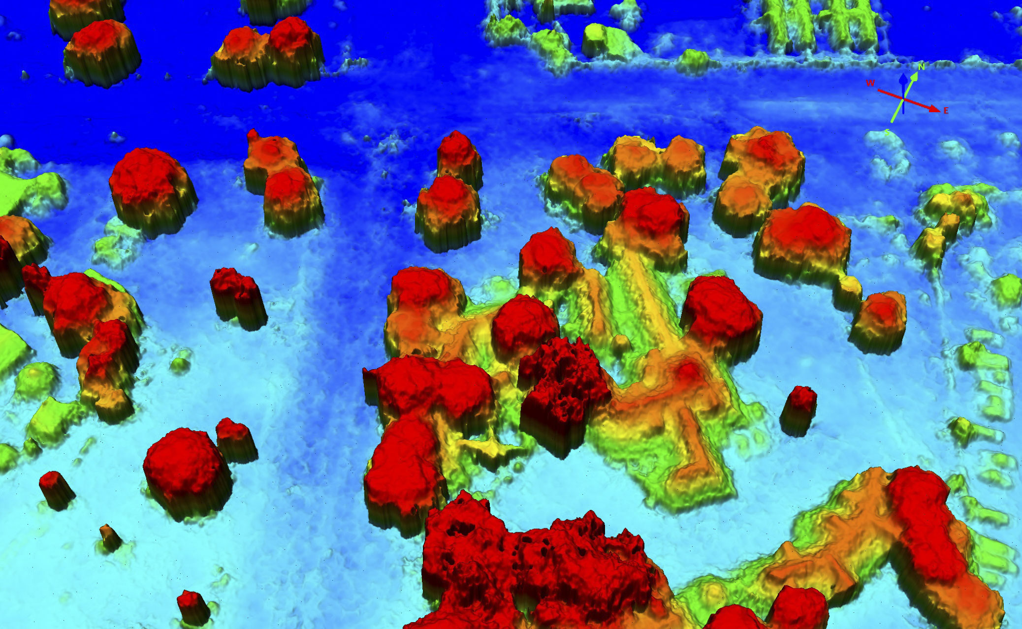
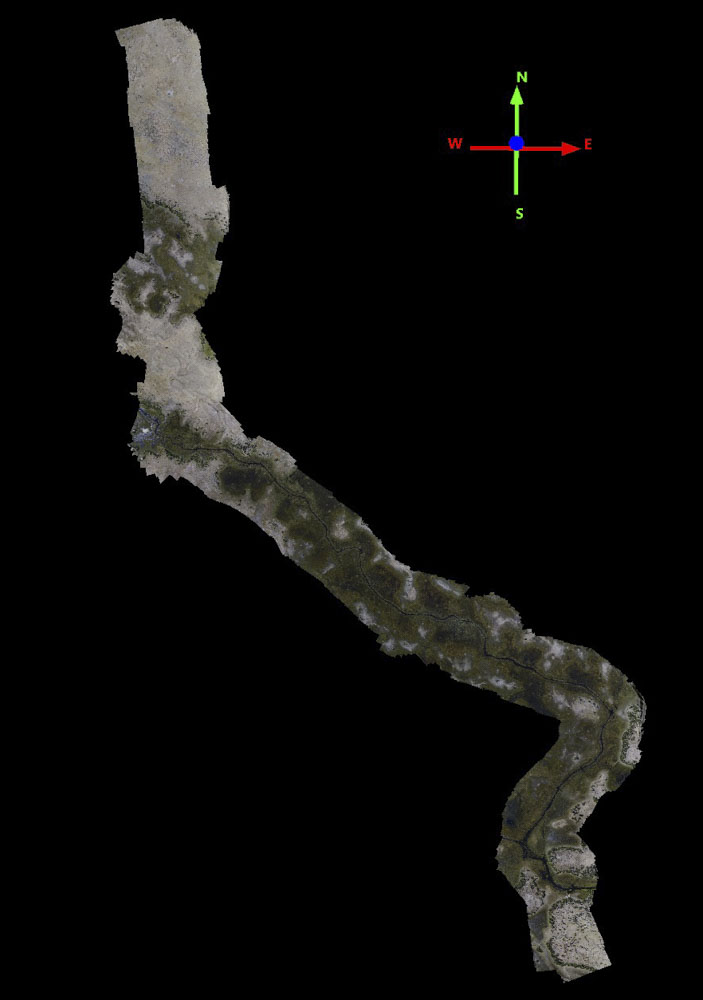
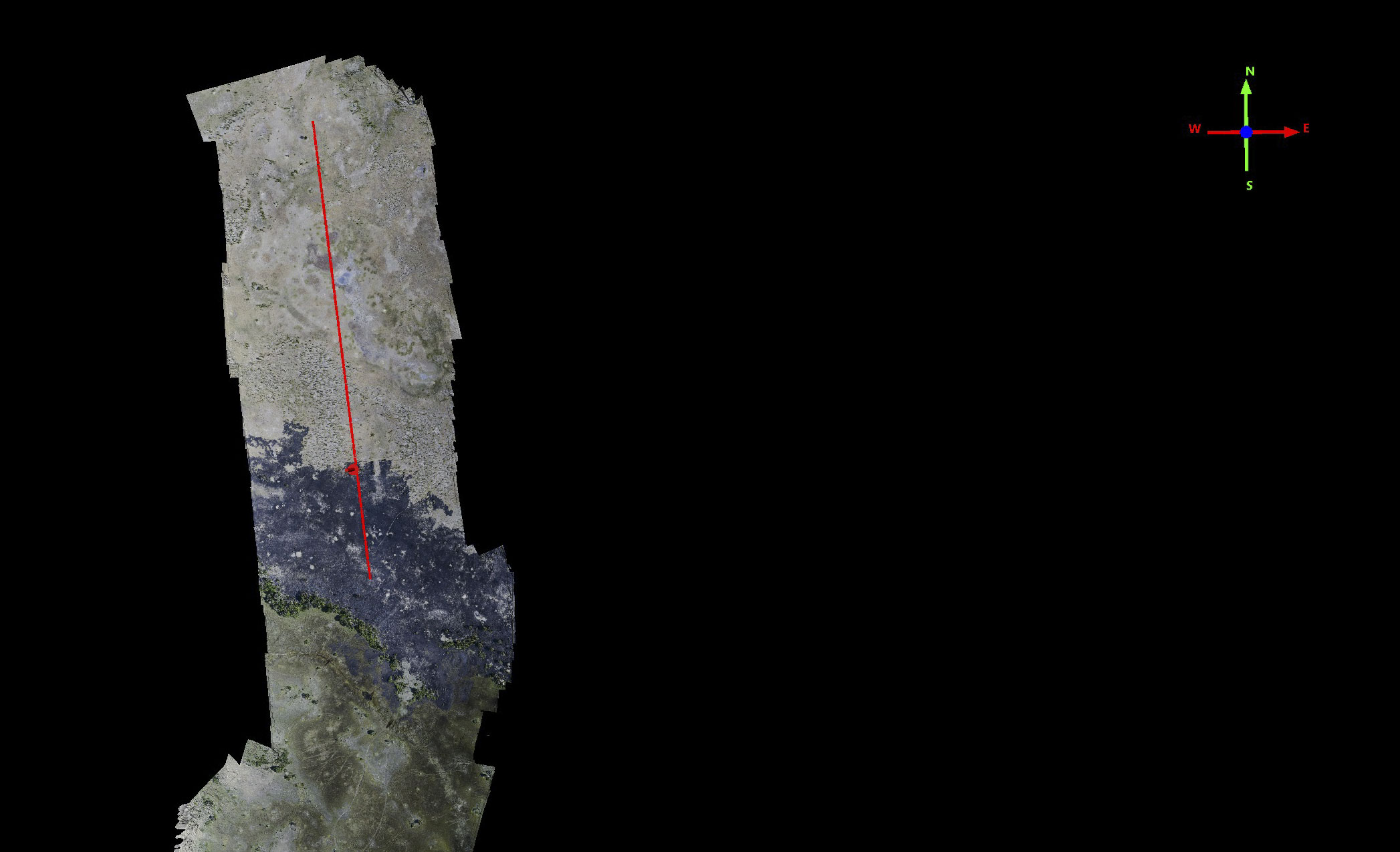
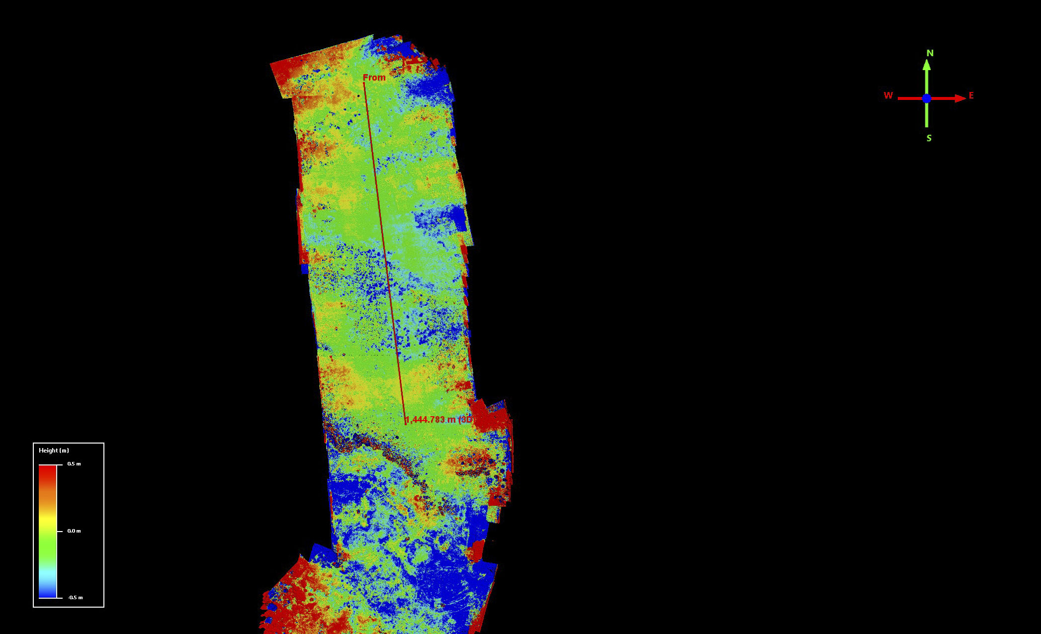
At left is the fodar orthoimage, at right the elevation data colored by height (blue low, red high). This transect is about 25 km long and 2 km wide.
Here is a circular fly-over of the point cloud of these data, at the north-eastern end near the river that flows into the swamp. Note that you can clearly see the size and shape of the trees, and even if they have sprouted leaves or not. We can make measurements of them all using the right software.
Kwando2 Block
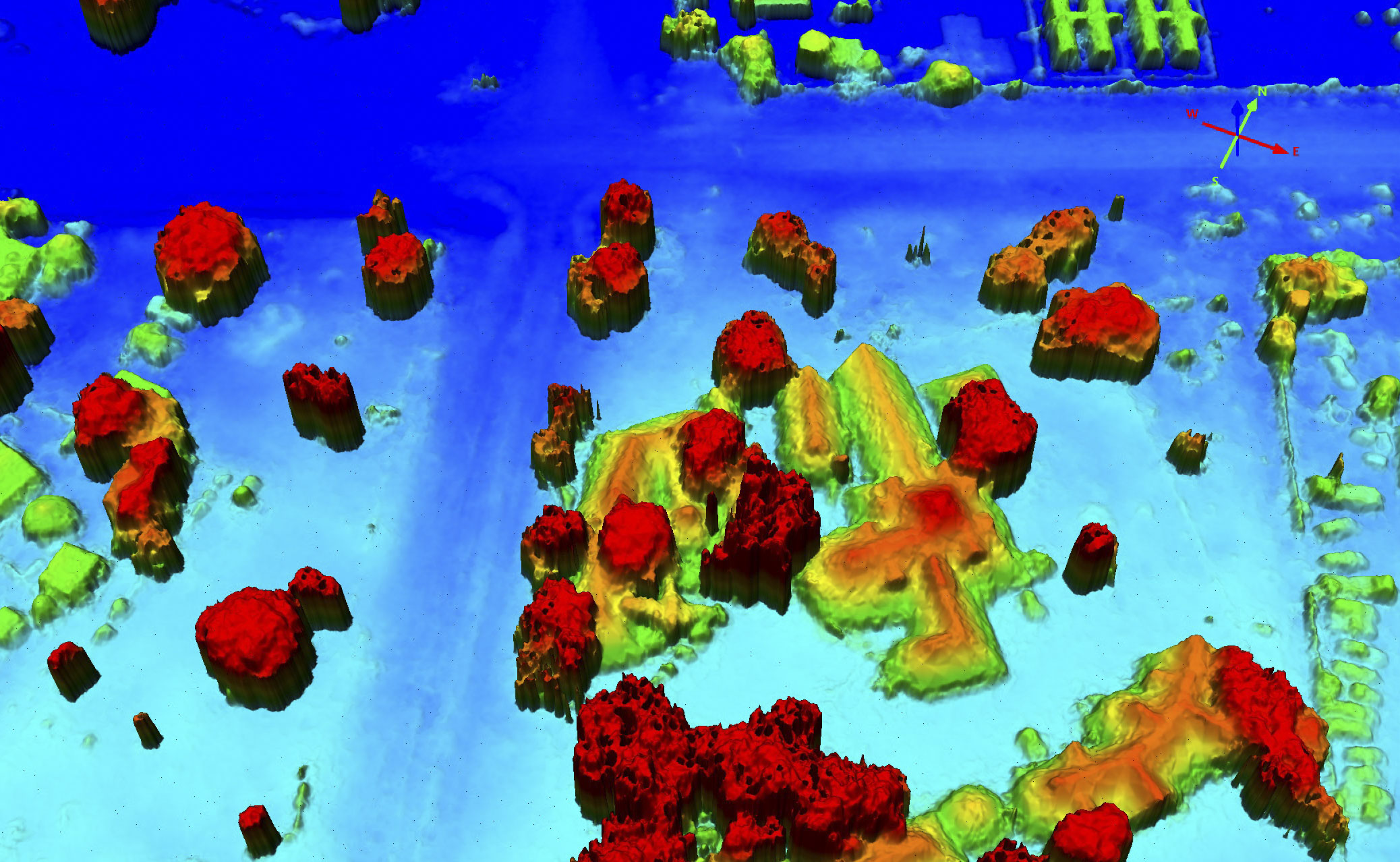
At left is the fodar orthoimage, at right the elevation data colored by height (blue low, red high). This transect is about 25 km long and 2 km wide.
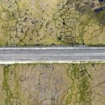
Here is a circular fly-over of the point cloud of these data, showing some of the fossil river channels. These channels filled with sand as they dried up millions of years ago due to subtle tectonic tilts in the landscape, and this sand now supports a vegetative community that differs substantially than the more clayey soils outside the channels. The red color is not clay, but rather leaf litter from the mopane trees that grow there; when we left in late November, the mopane were just begin to leaf out.
CH1 Block
At left is the fodar orthoimage, at right the elevation data colored by height (blue low, red high). This transect is about 25 km long and 2 km wide.
Here is a 3D visualization of these data demonstrating the transitions in vegetation type cause by subtle drainage differences. We can measure both the vegetation and the topography using these data to understand these relationships better than ever before.
NG18A Block (including CSU camp)
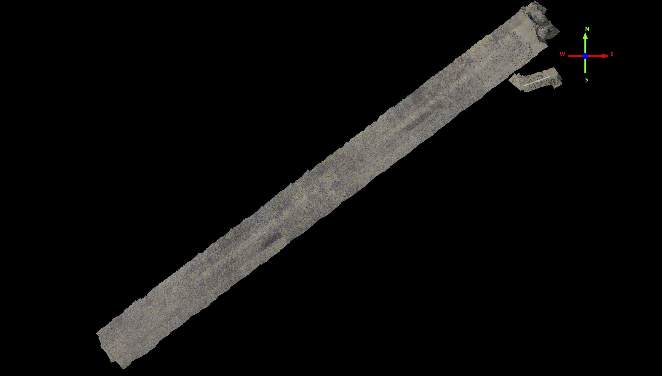
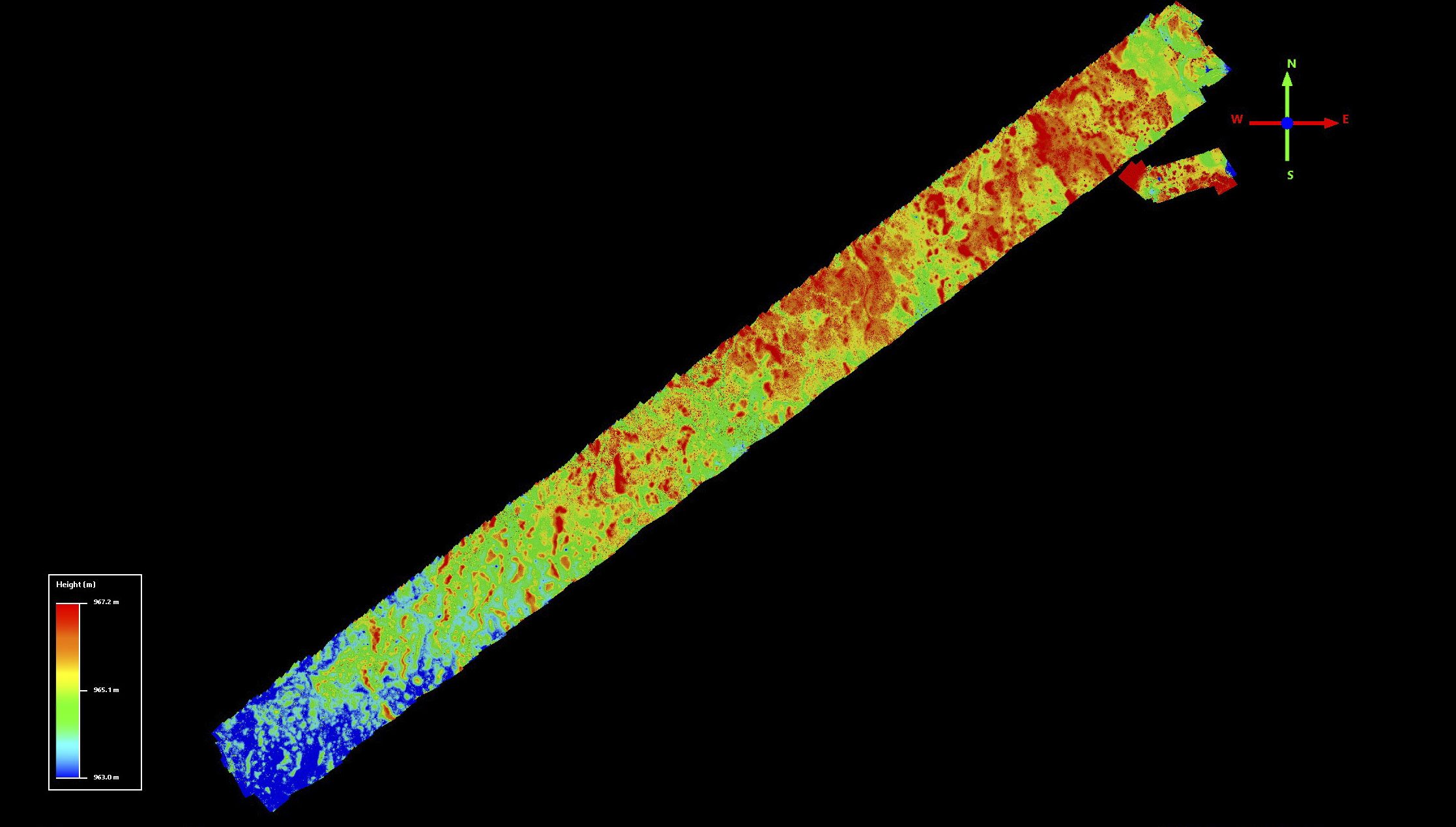
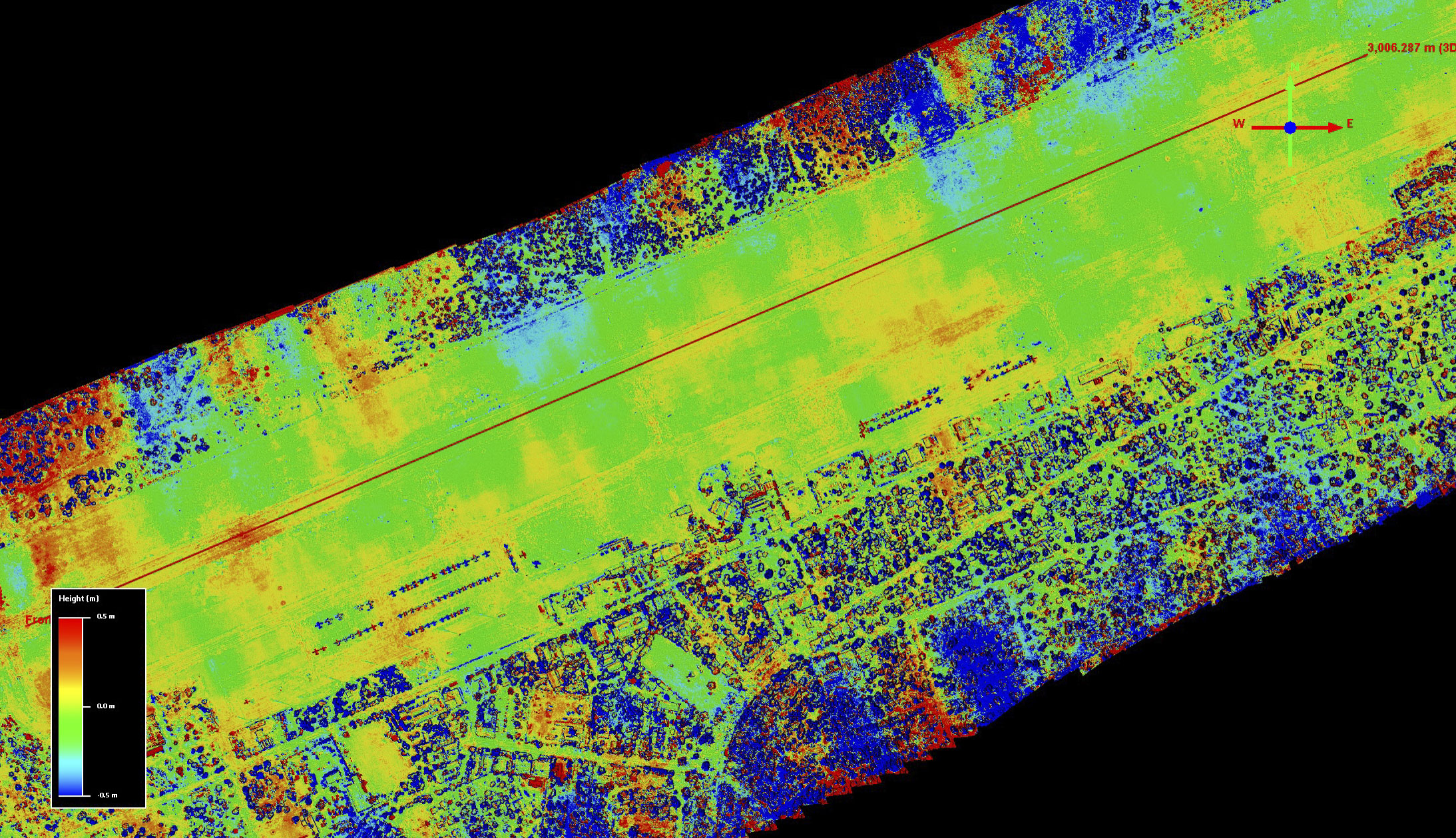
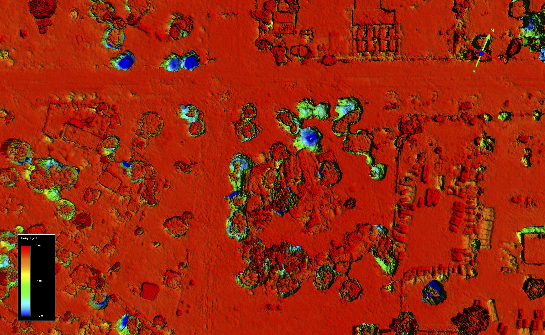
At left is the fodar orthoimage, at right the elevation data colored by height (blue low, red high). This transect is about 50 km long and 2 km wide.
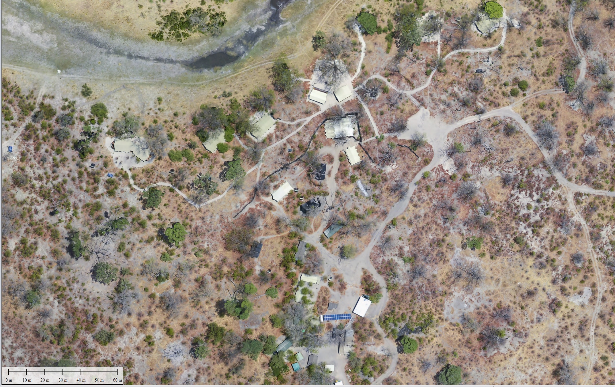
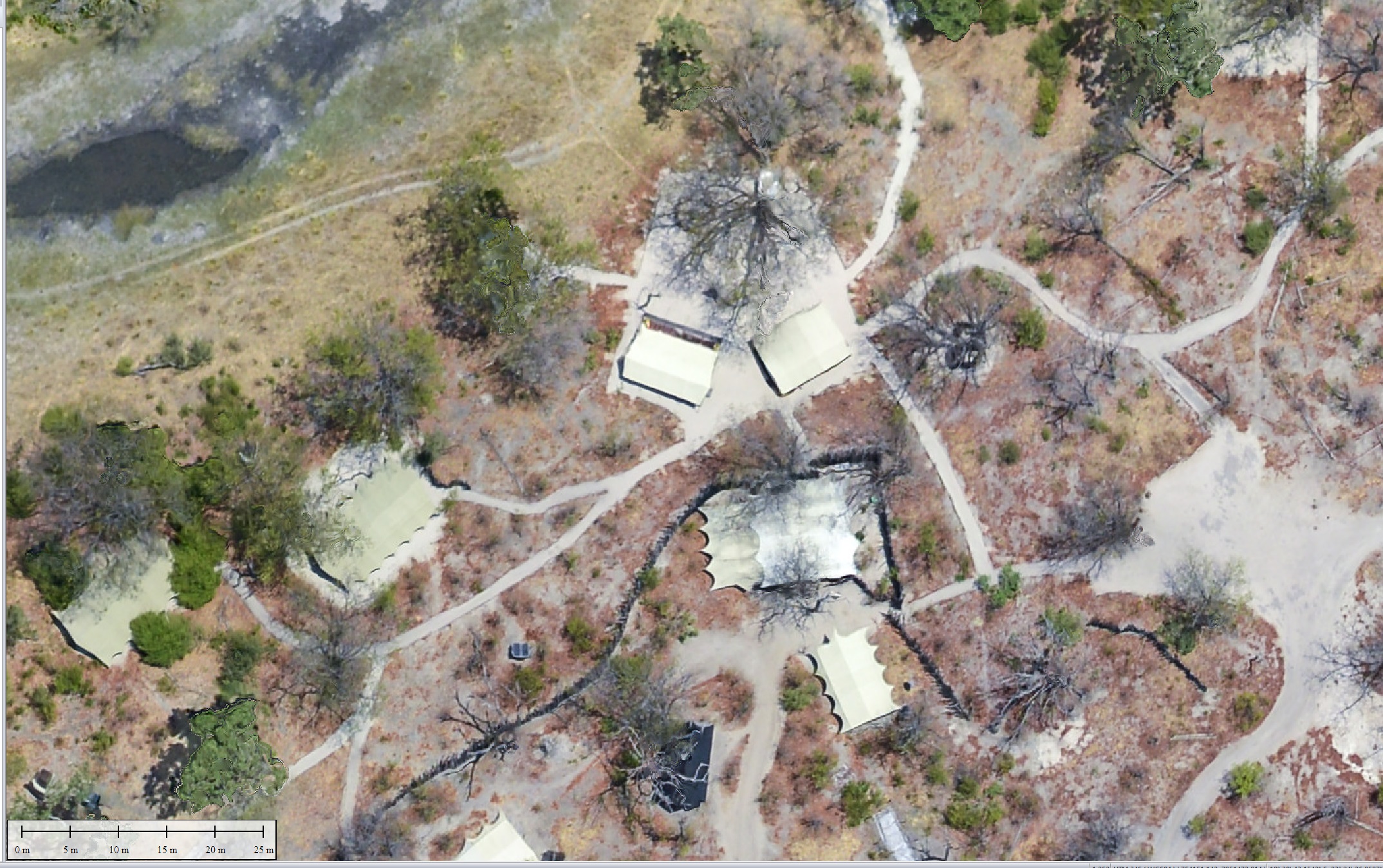
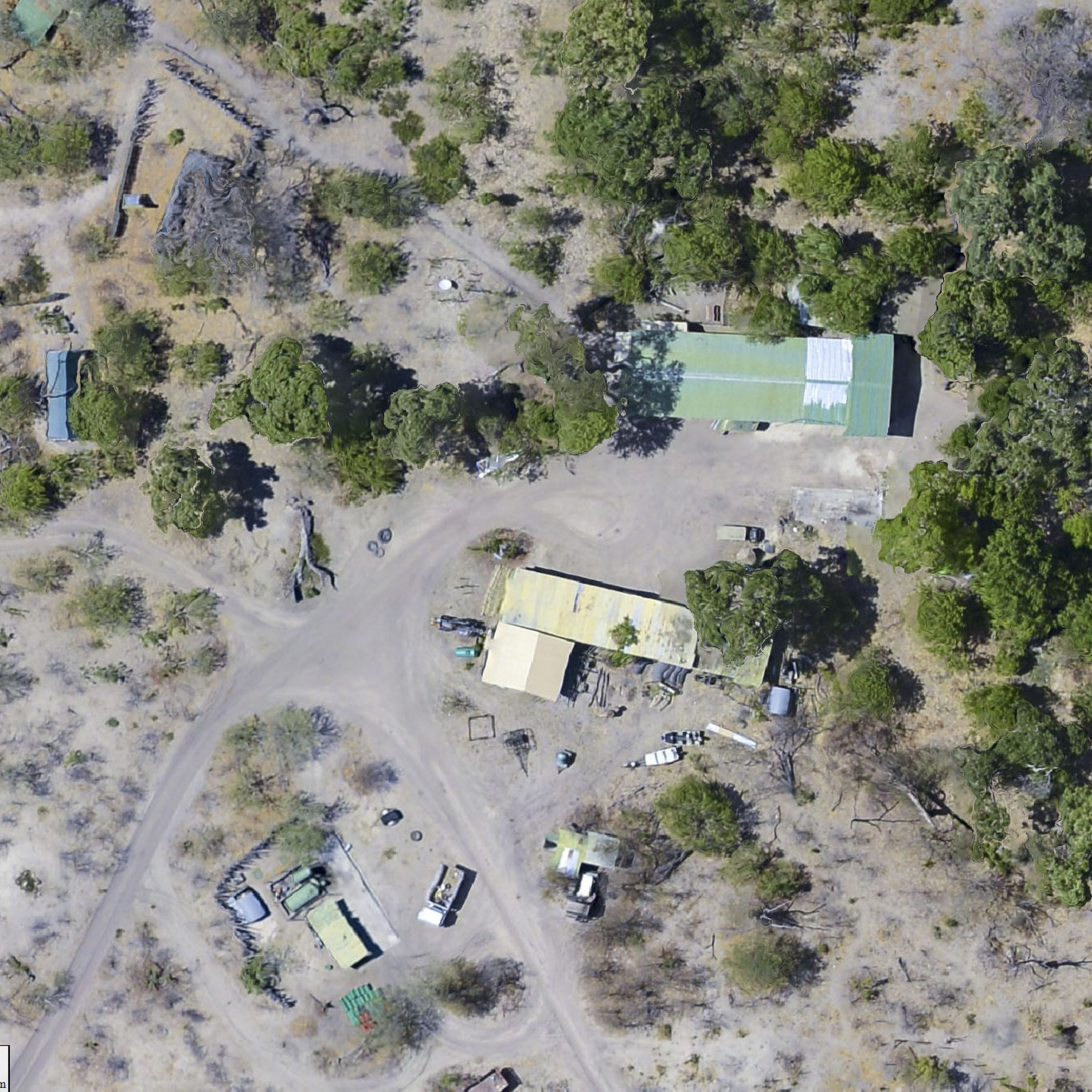
Here is a 3D visualization of the point cloud of these data circling around CSU camp at the northern end of the block. The broad parallel tracks to the north of camps are one of John’s experiments to increase forage and habitat for non-woodland creatures in the area.
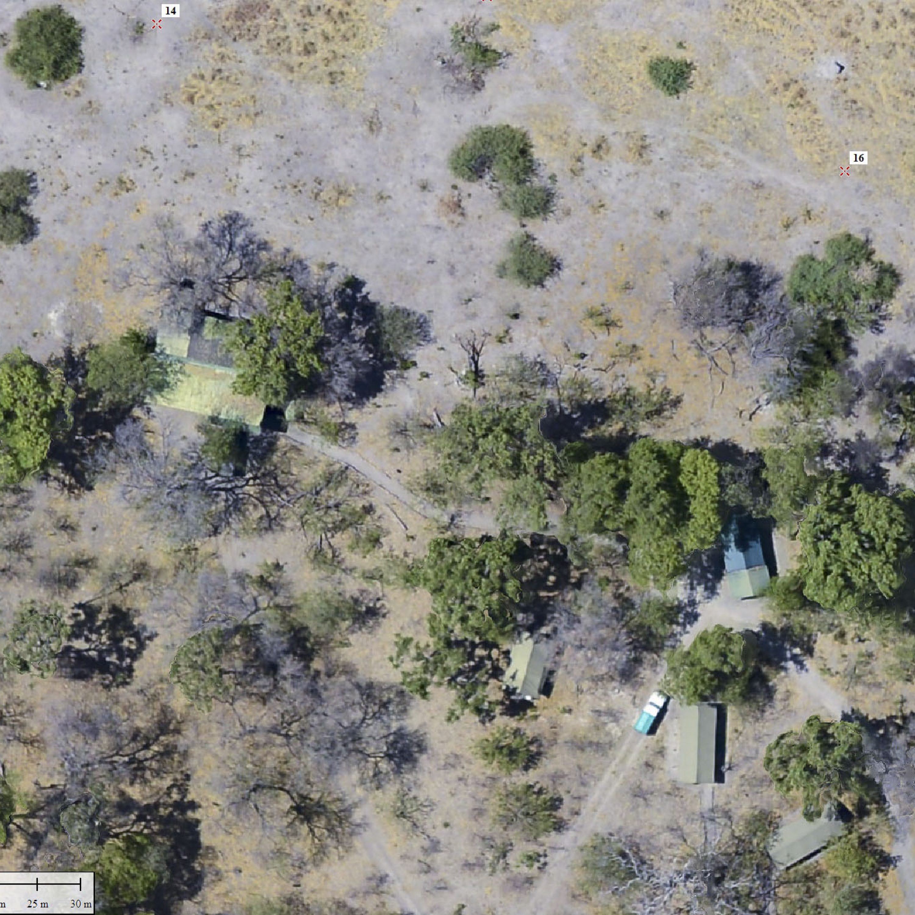
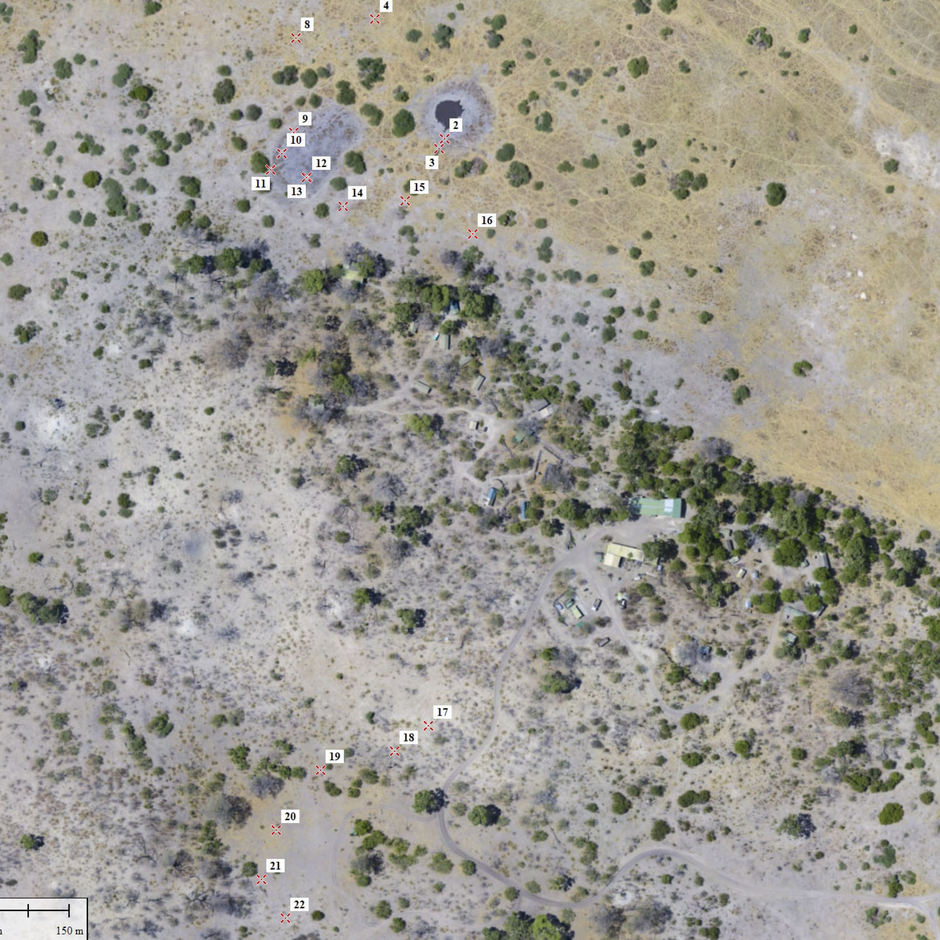
Here is a closeup of the orthoimage showing CSU camp. Our tent was just to the left of the white truck. The numbers near top are some of my ground control points for the project, described later.
Spillway Block (including Selinda Spillway and Savute Channel)
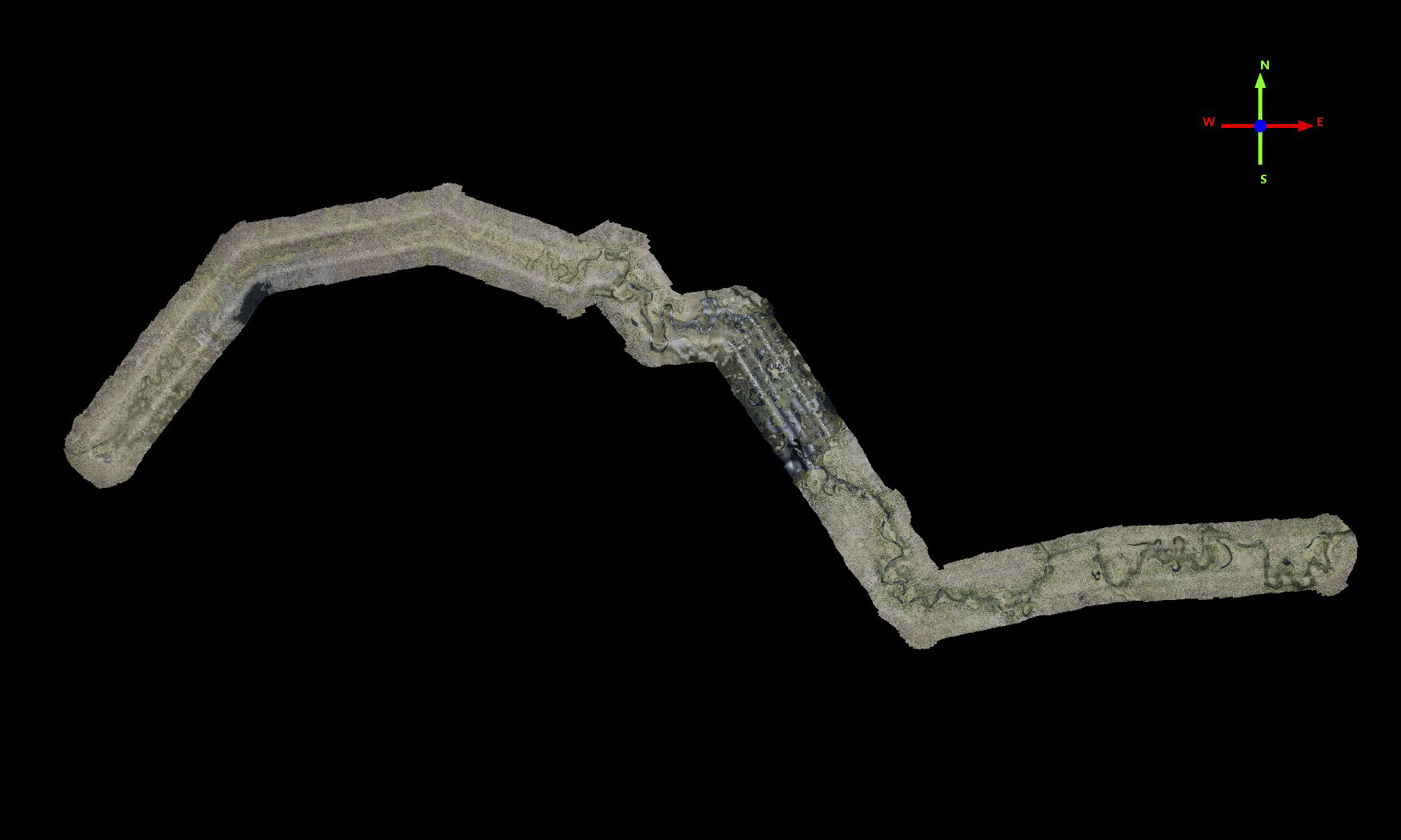
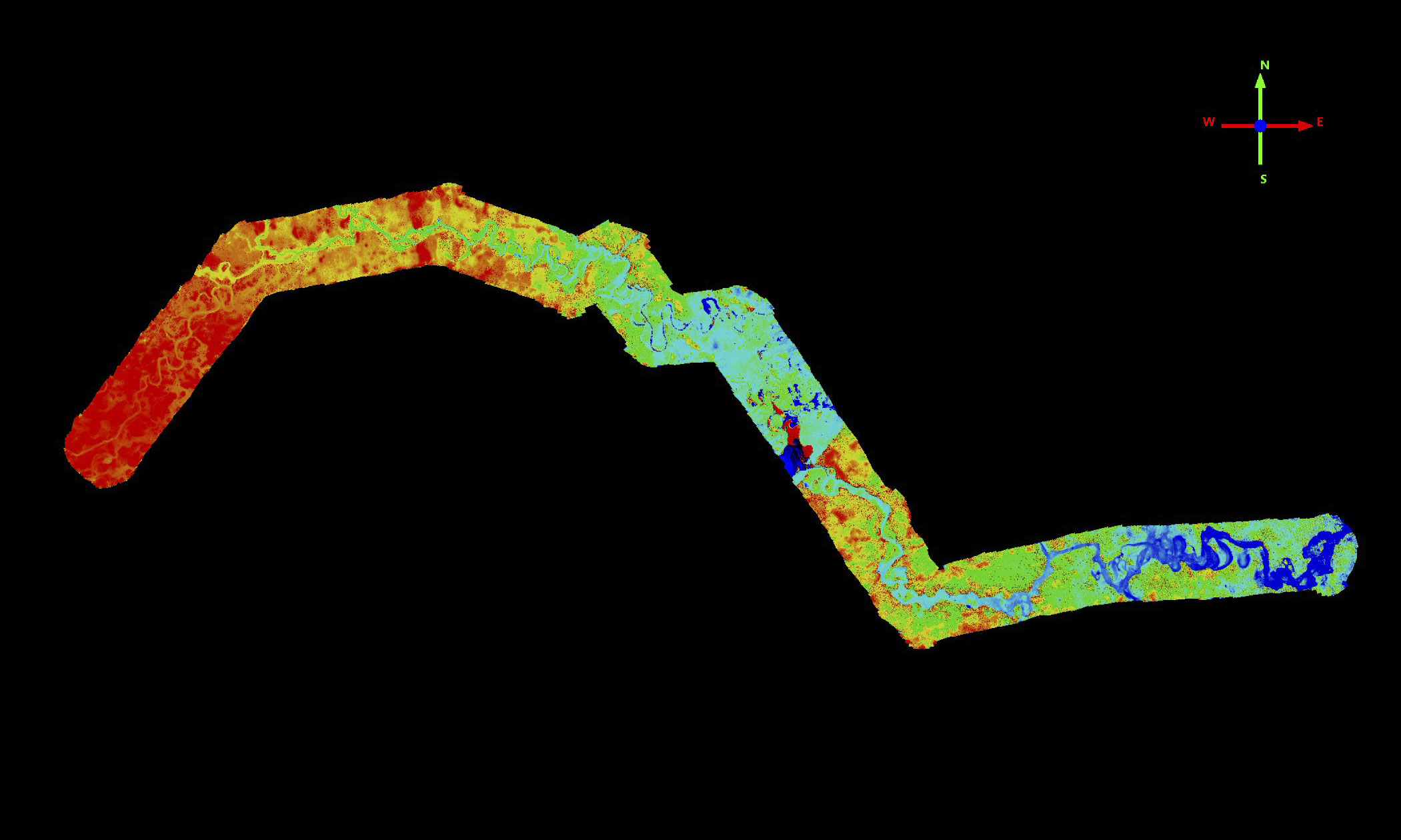
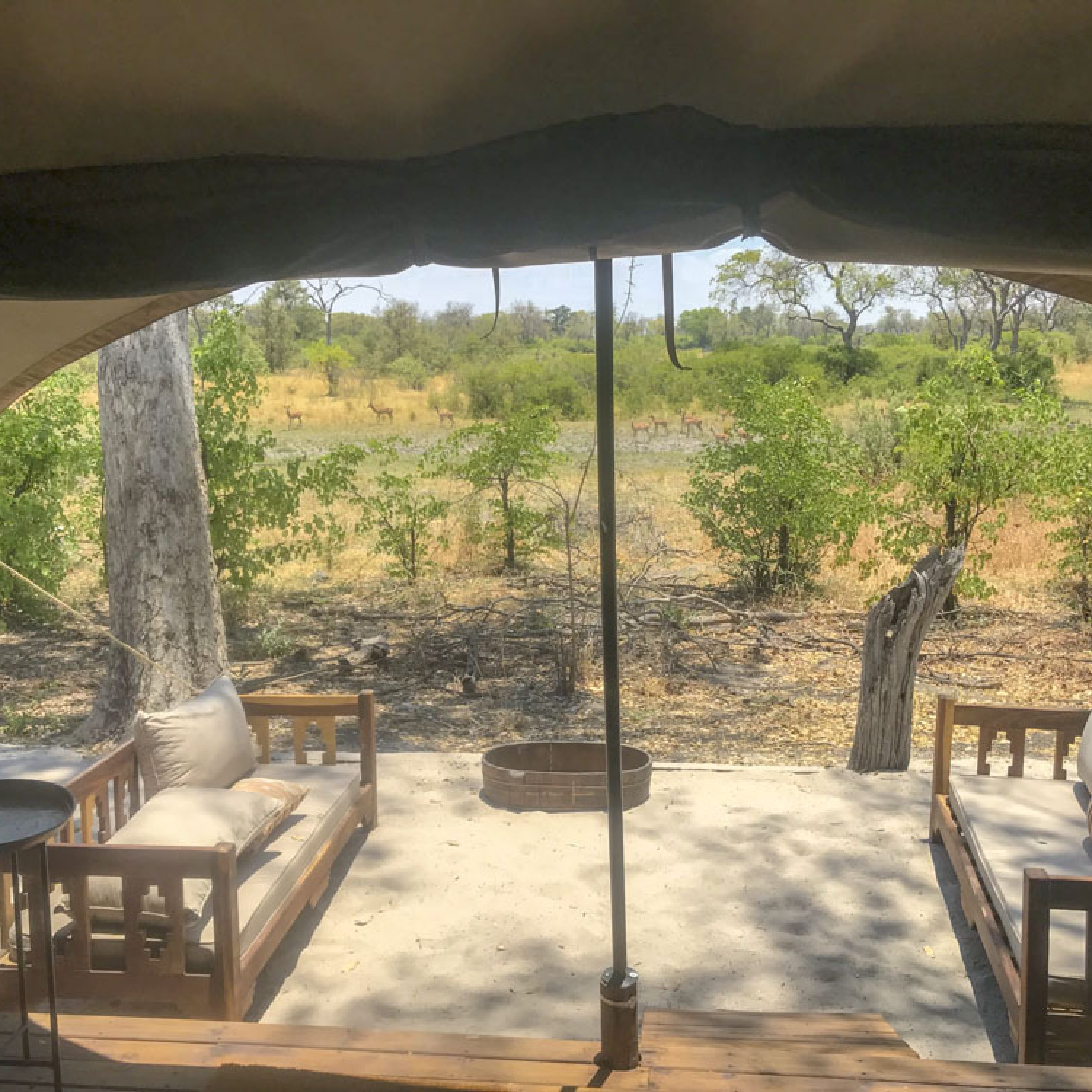
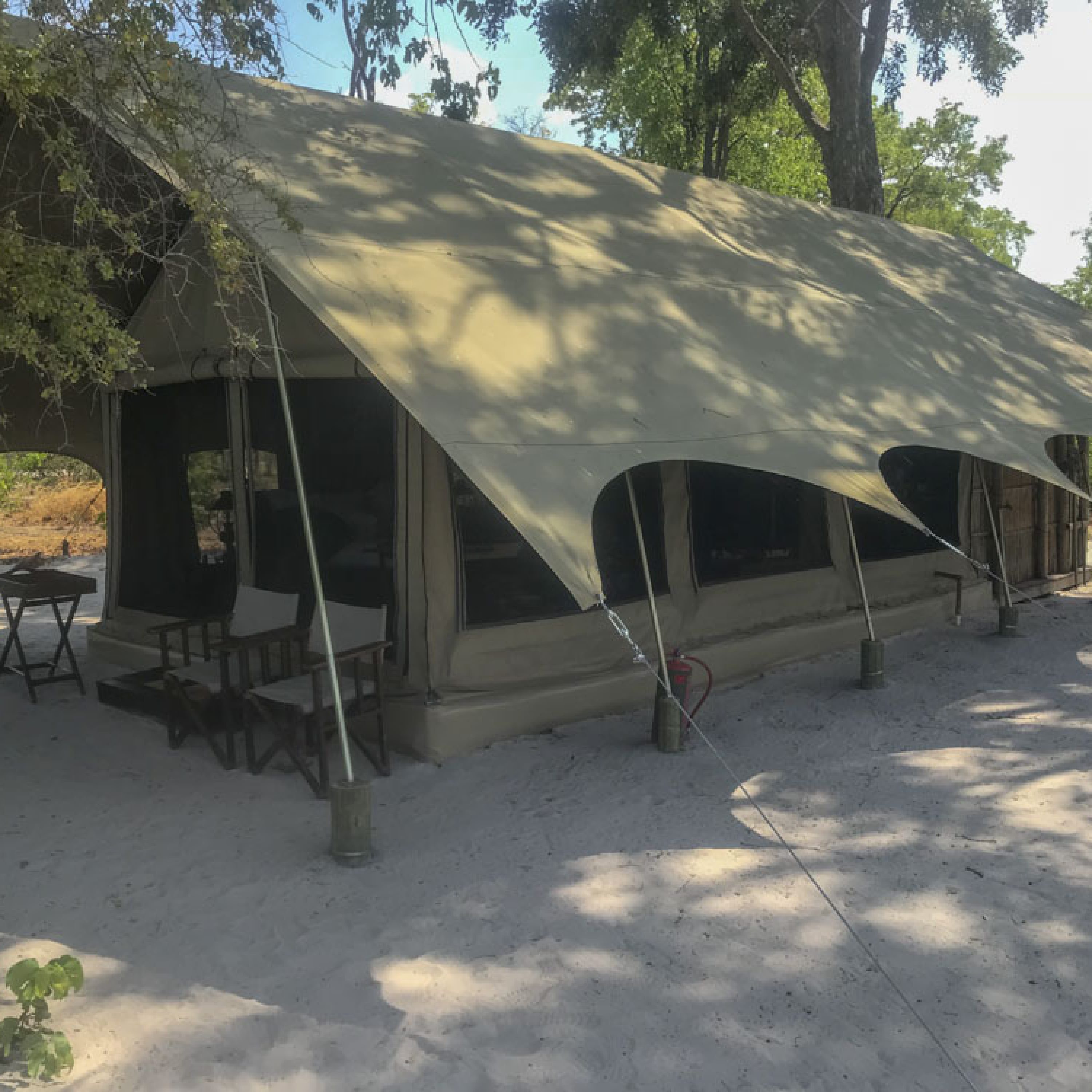
At left is the fodar orthoimage, at right the elevation data colored by height (blue low, red high). Here is Selinda Explorer’s Camp, an excellent camp run by Great Plains Conservation. We stayed in the huge tent at left and in one at upper right (we booked only a week before our trip and were happy to take any tent available!). Because the images are orthorectified, then can be used for making accurate measurements.The main lounging area is at top center, open-sided tents with couches and cushions for relaxing. The large leafless tree there is next to an enormous termite mound.
Here is a 3D visualization of the point cloud of these data around the tip of the Linyanti swamp. It’s just such a cool area, I could spend hours flying around on these data or weeks flying around it for real and not be bored.
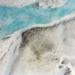
Here is a 3D visualization of the 2018 fodar data flying us from the Linyanti swamp into the Savuti Channel, a fascinating drainage feature with millions of years of interesting tectonic-hydrologic history to explore. Note how well the water itself is resolved due to the floating vegetation, such that we can easily measure water levels and gradients.
NG18B Block
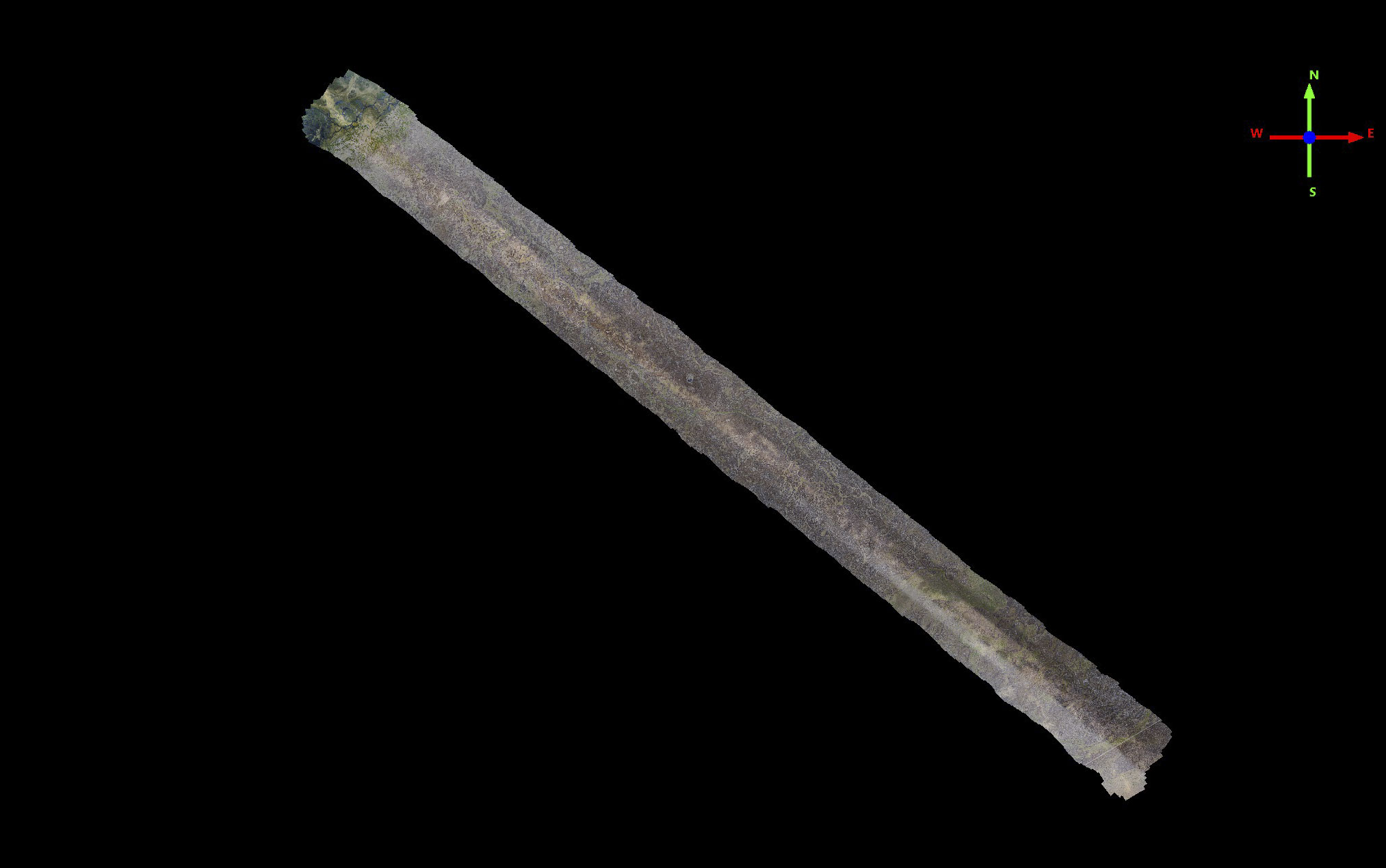
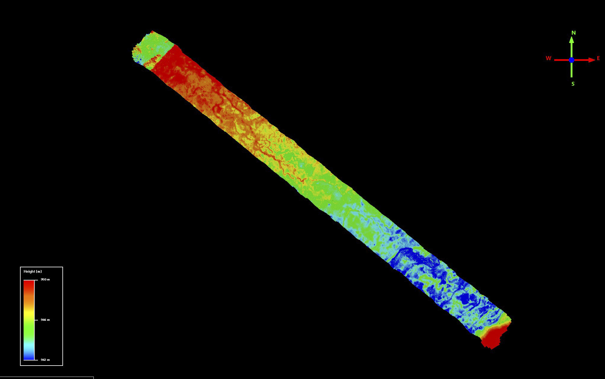
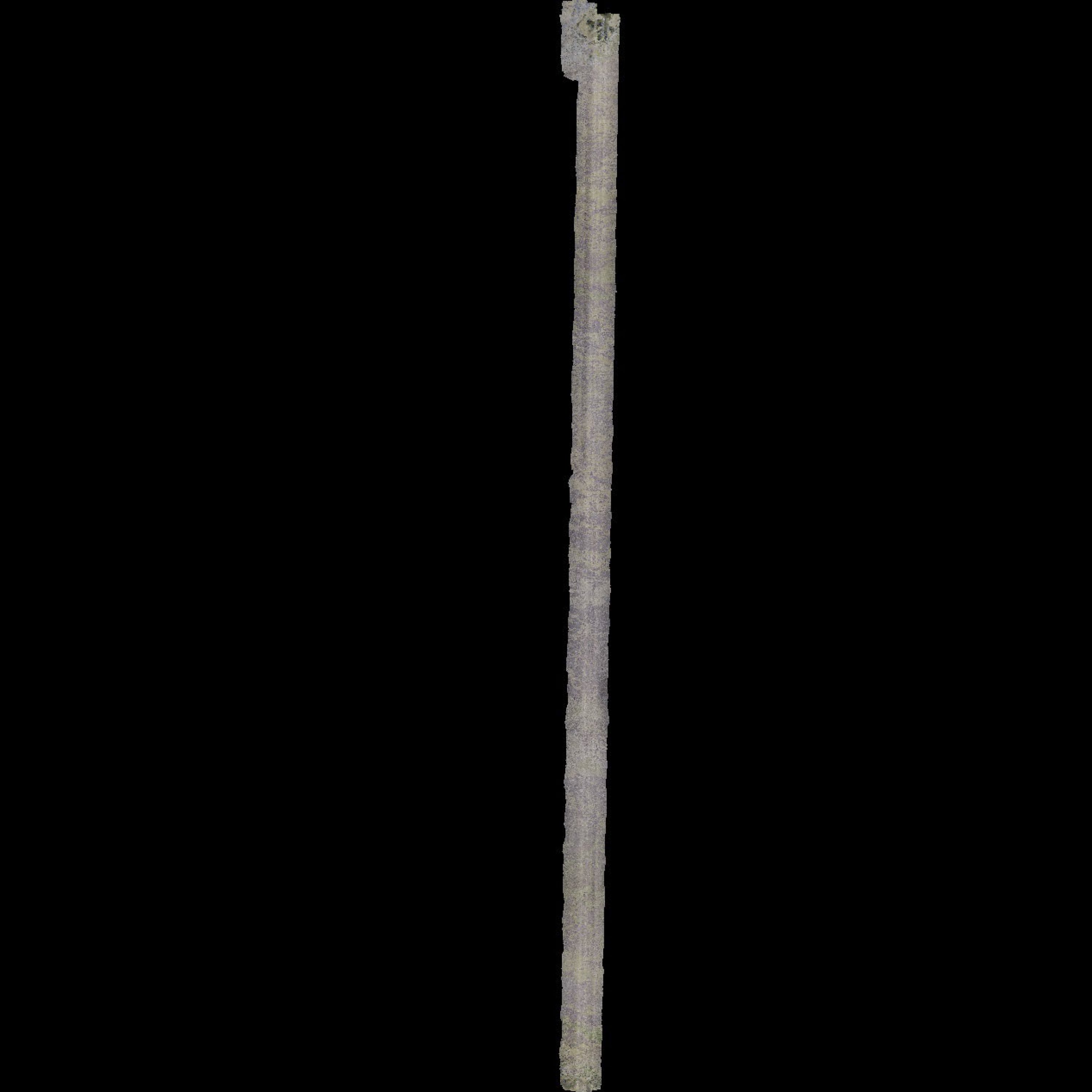
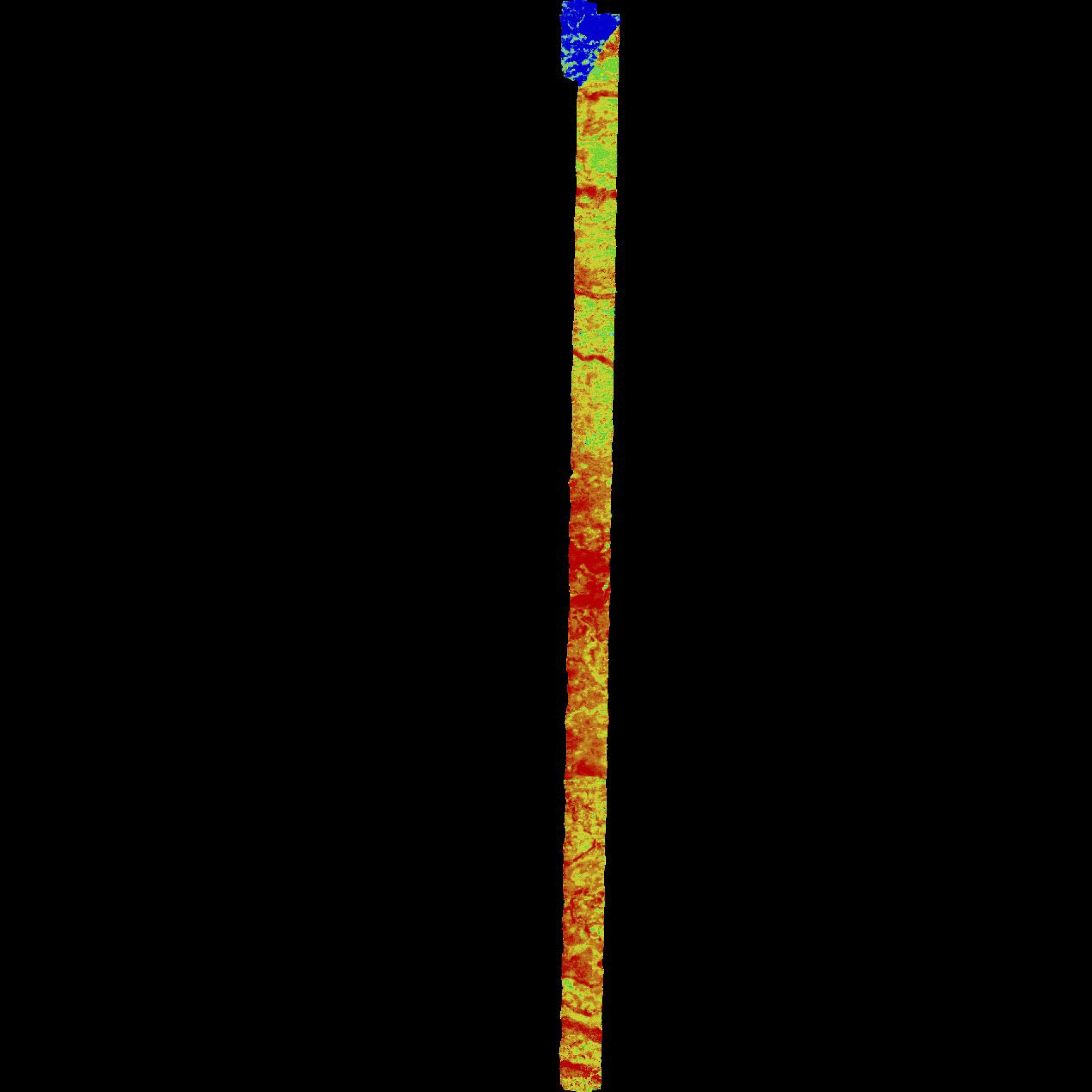
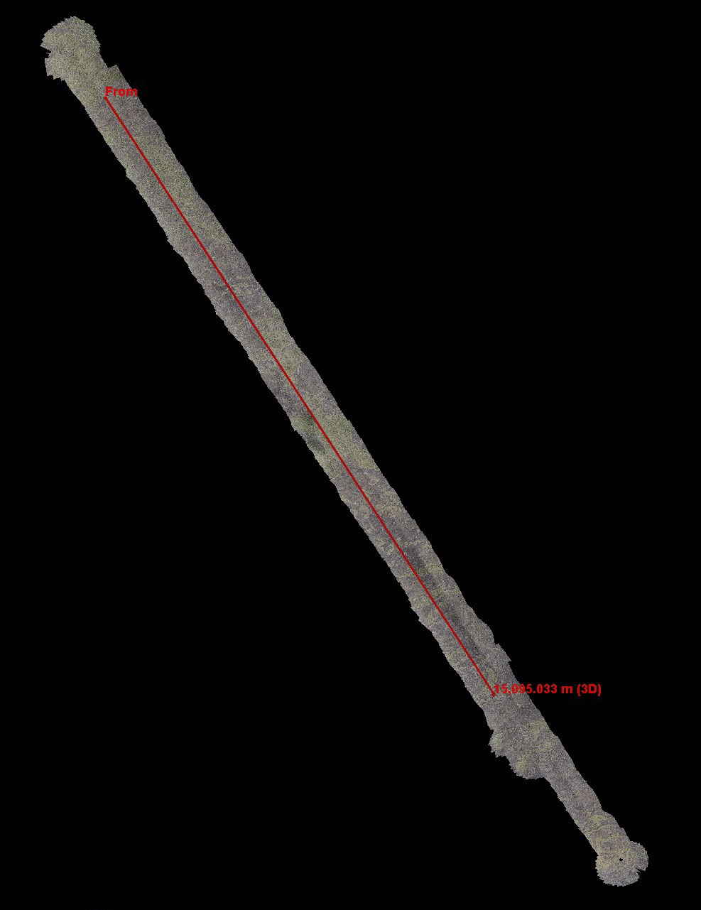
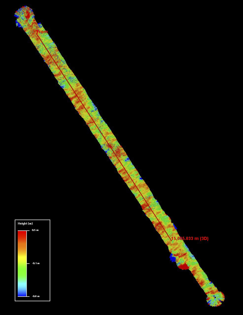
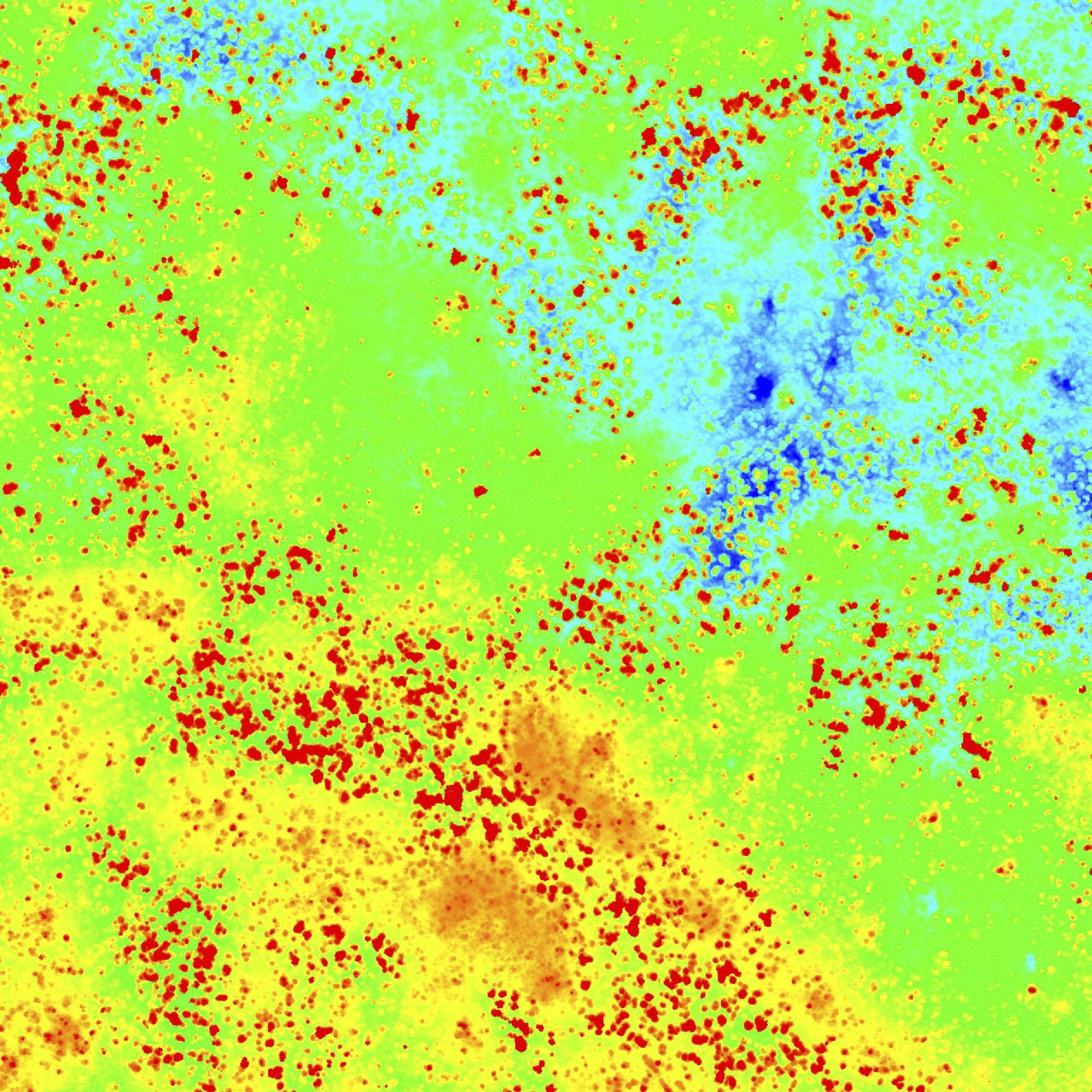
At left is the fodar orthoimage, at right the elevation data colored by height (blue low, red high). This transect is about 25 km long and 2 km wide.
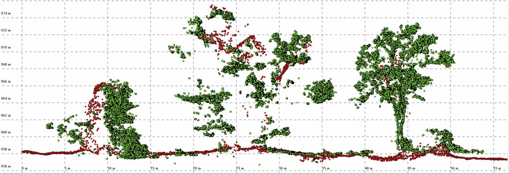
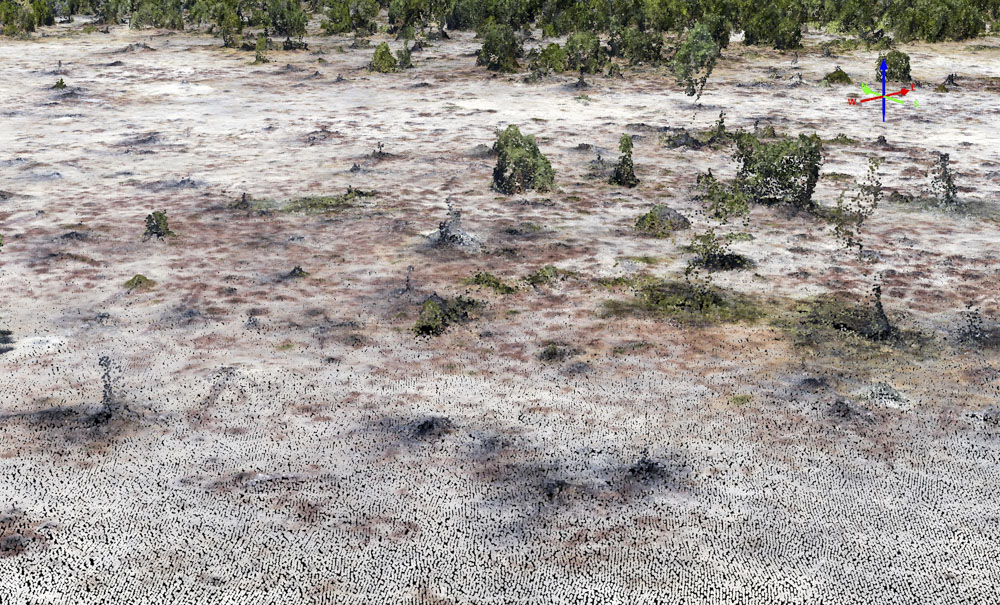
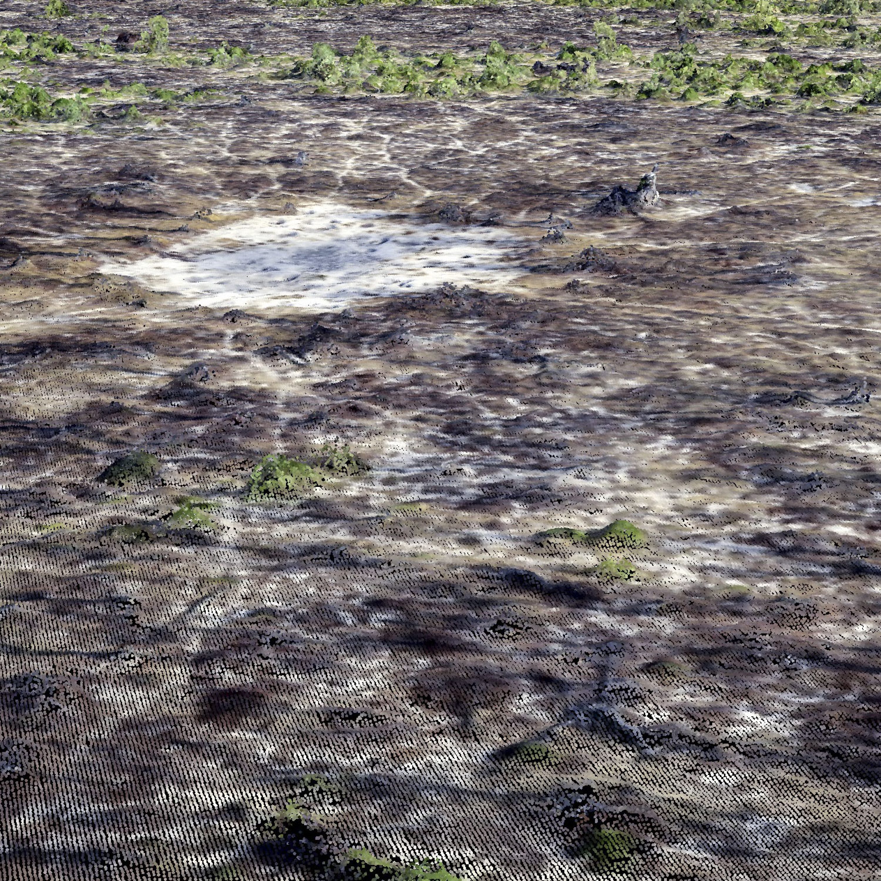
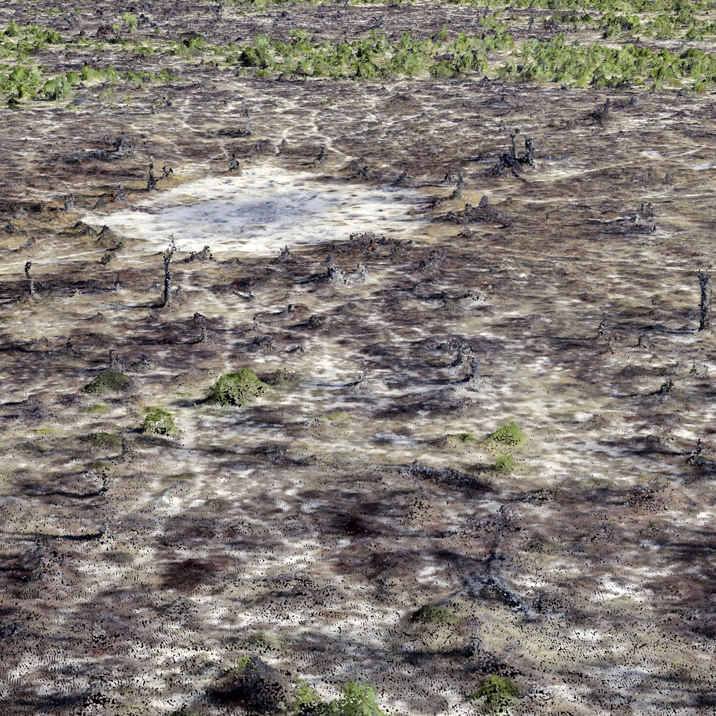
Here is a 3D visualization of the point cloud of these data circling around a mopane forest which has been stunted due to severe elephant browse. The leaves had yet to sprout when we mapped it, making it look lead it was all dead at first glance.
Accuracy and Precision Checks
The project itself was way underfunded so there was no budget at all for ground control or data validation, but we were able to sneak some in any way. Validation here is really mostly for blunder checking, I did a thorough validation of the 2017 Botswana data and many other validation projects here. The two basic tests I used were comparing the fodar maps to those I made in 2017 and using survey-grade GPS on the ground. Here I was mostly only able to really nail horizontal accuracy, as my field book was lost/stolen (first time in 25+ years!) within a few minutes of arriving back in Maun so I don’t have exact antenna heights to check vertical. In any case, horizontal precision/accuracy seems to be better than 1-2 pixels (10-20 cm) and vertical precision is < 20 cm at 95% as we’ve always found, and vertical accuracy is likely better than 30 cm but no worse than 2 m (due to possibly blunders); a few high quality GCPs in each location can be collected at any time to resolve any blunders.
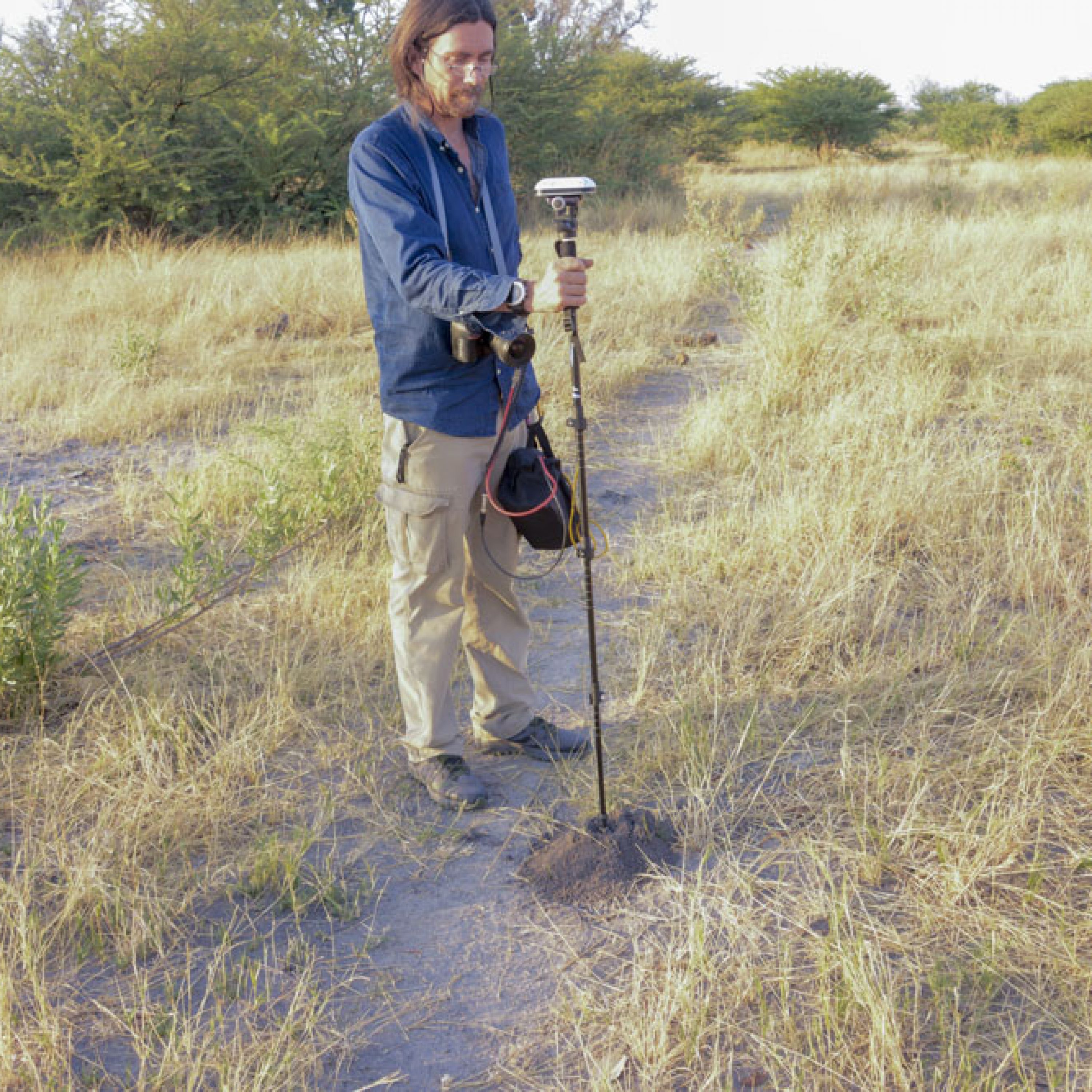
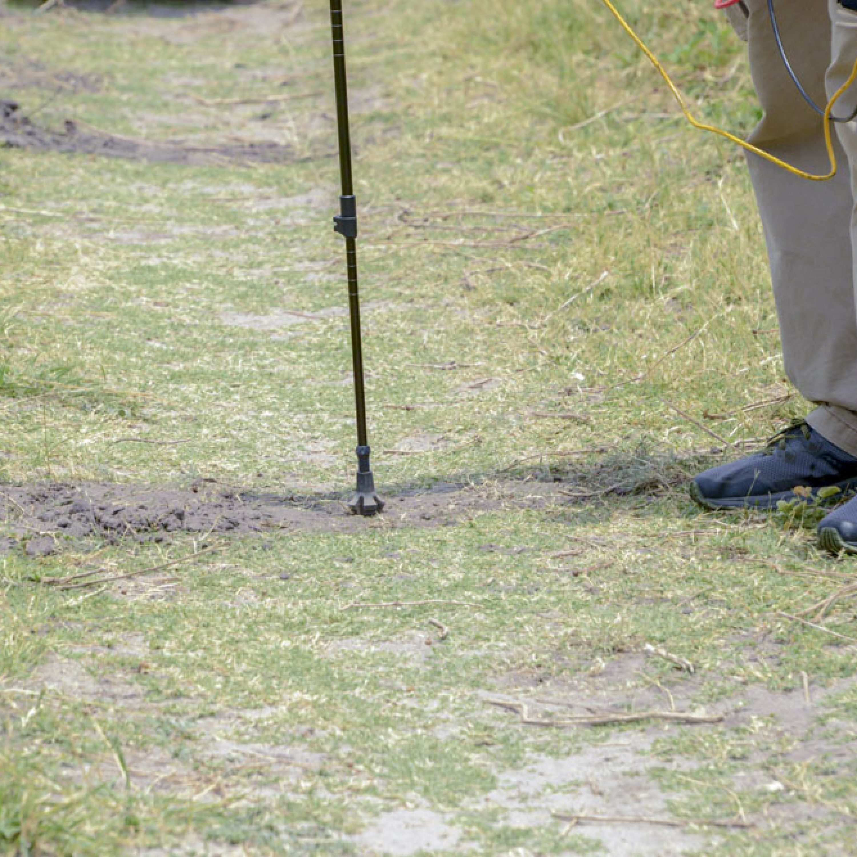
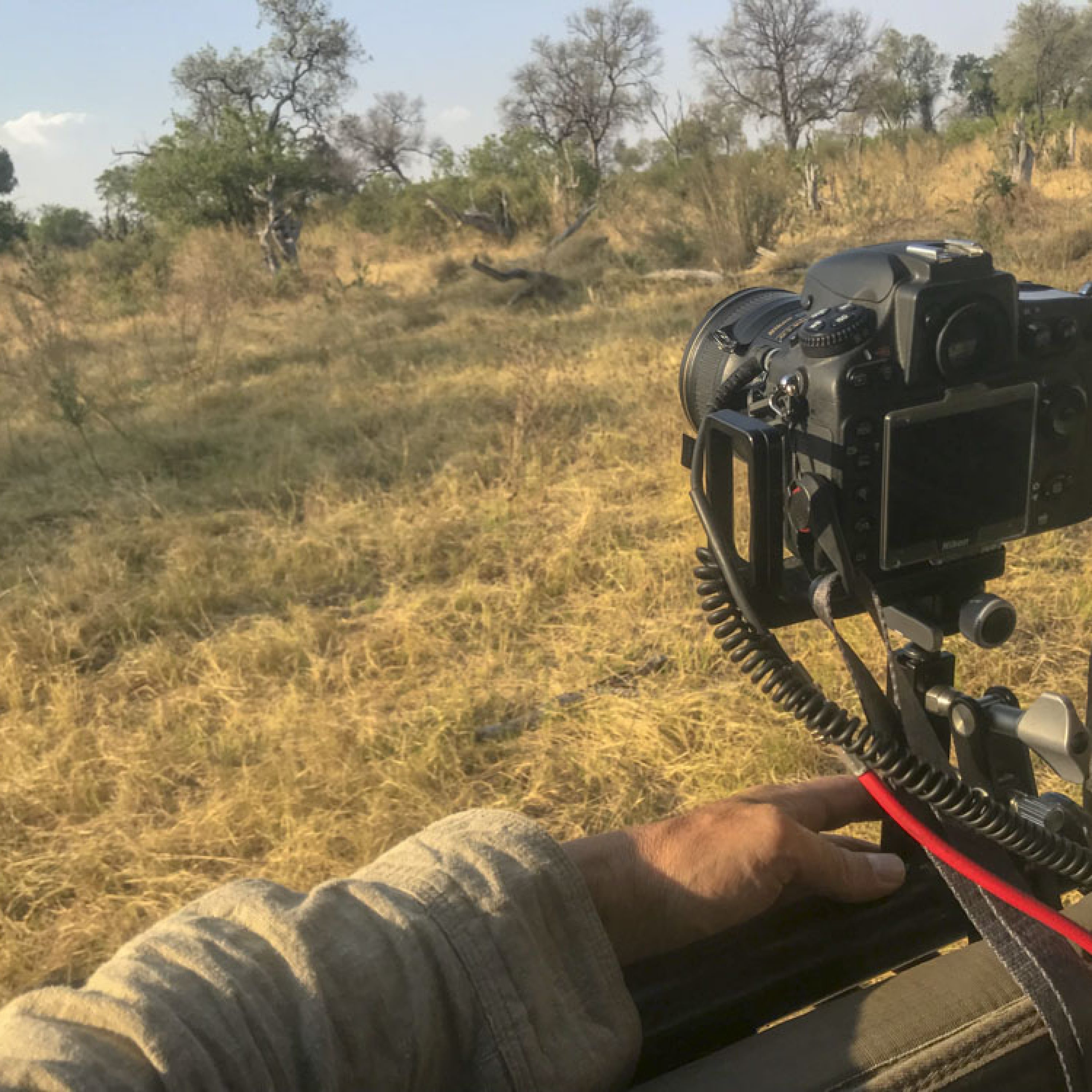
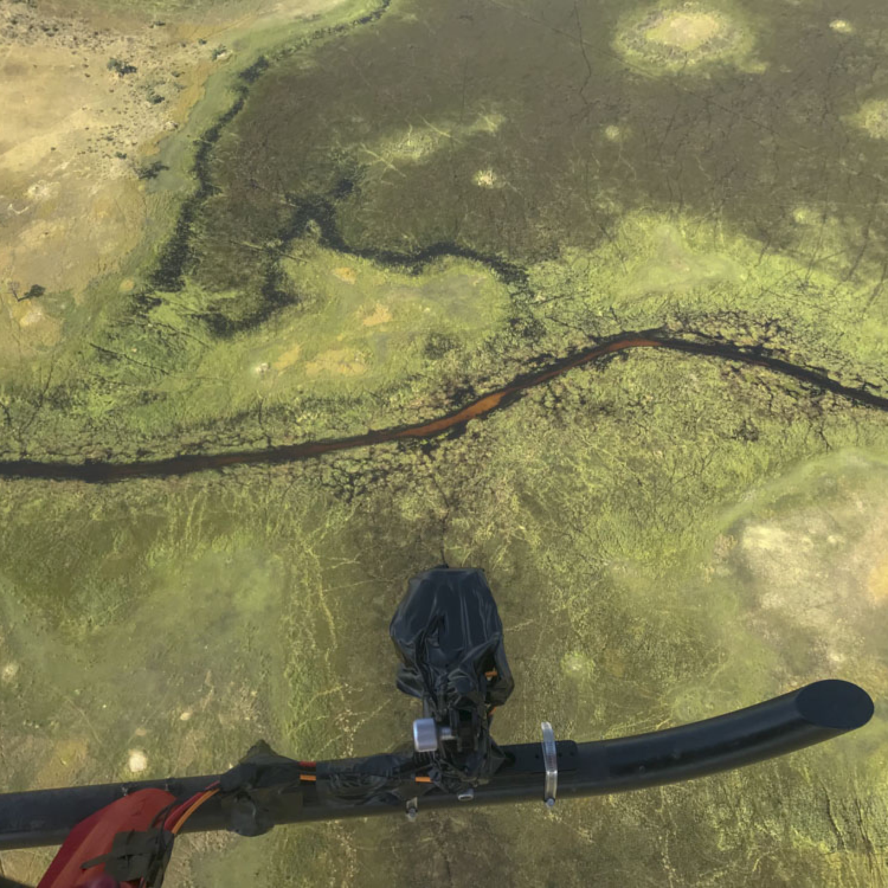
However the major point of this field work for me was as a methods test for measuring ground control in Botswana itself, rather than validation for the airborne data which I’ve validated countless times now. Along these lines I was able to collect some survey-grade GPS data based from CSU camp and Selinda Explorer’s camp several weeks later by adapting my airborne system for walking and vehicle use, progressively getting more sophisticated. First, early in the morning before we left CSU camp to return to Maun, we mounted the aircraft antenna to a monopod and walked around camp surveying ground features that might be visible in our maps, while Turner followed behind taking photos of the features I was surveying. Next we mounted the antenna onto the hood of a safari vehicle and made continuous measurements; I had some issues with that in our drive from CSU camp (partly due to overhanging canopies), but had them sorted for the others. Then I began acquiring oblique fodar data, by mounting the camera to the truck and taking bursts of photos obliquely at the scenery such that we could make points clouds from the ground for comparison with those made in the air. Finally on our self-drive trip we simply drove through the southern end of NG18A and took geolocated photos without the survey system as a means to validate our species identification from the fodar orthomosaics, using techniques that could be done by anyone without expensive gear.
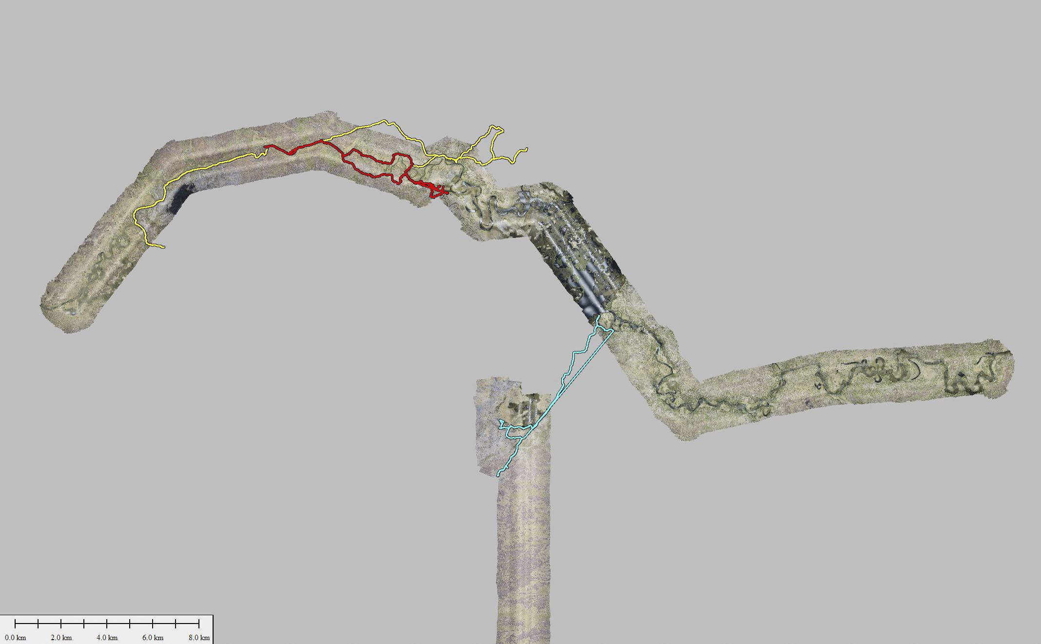
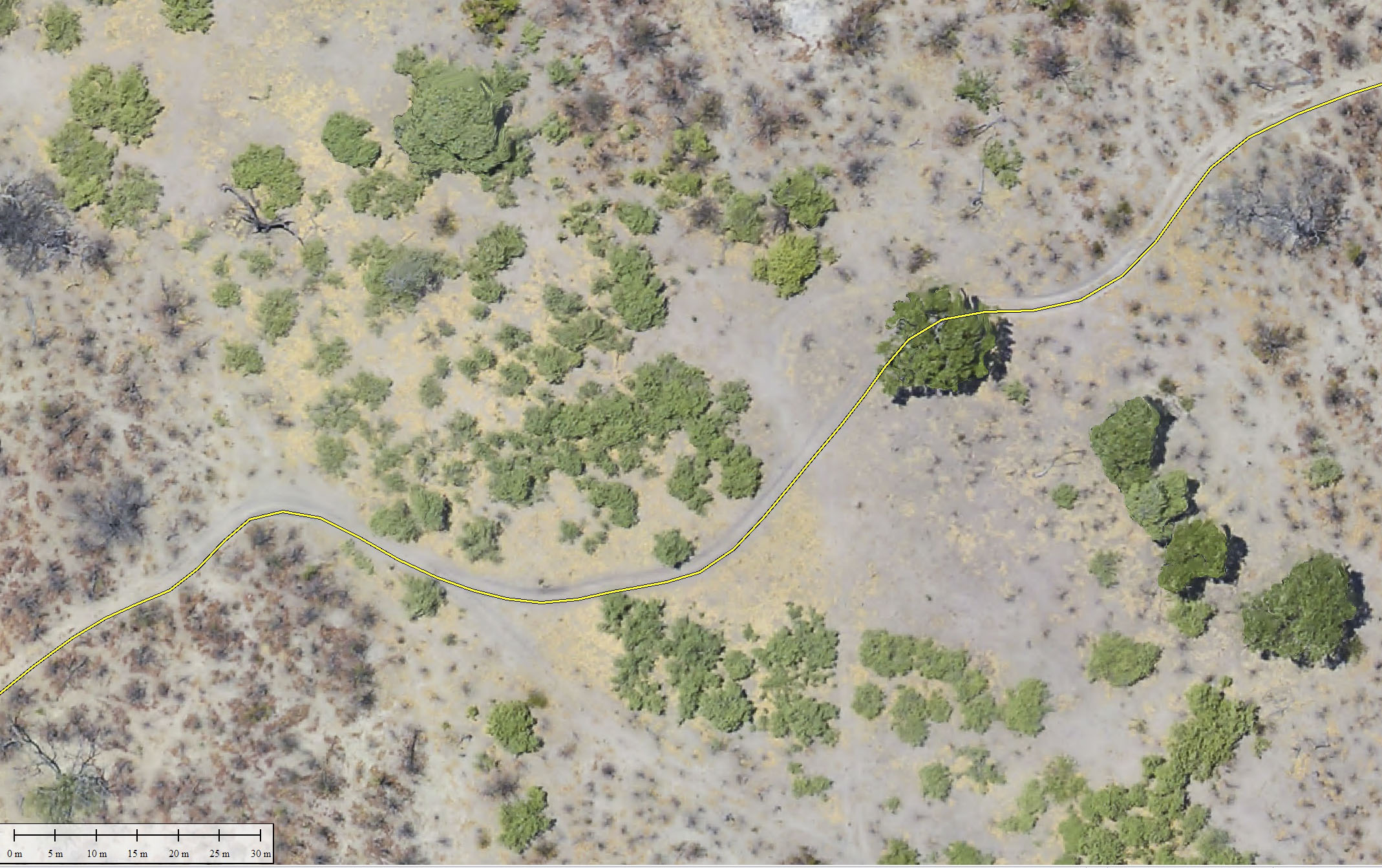
Here are our driving tracks overlaid onto the Spillway Block and NG18A blocks, with those from CSU camp in blue and Selinda Explorer’s camp in red and yellow lines. The self-drive tracks are not shown here, but are at the bottom of the cut-off NG18A transect shown here.
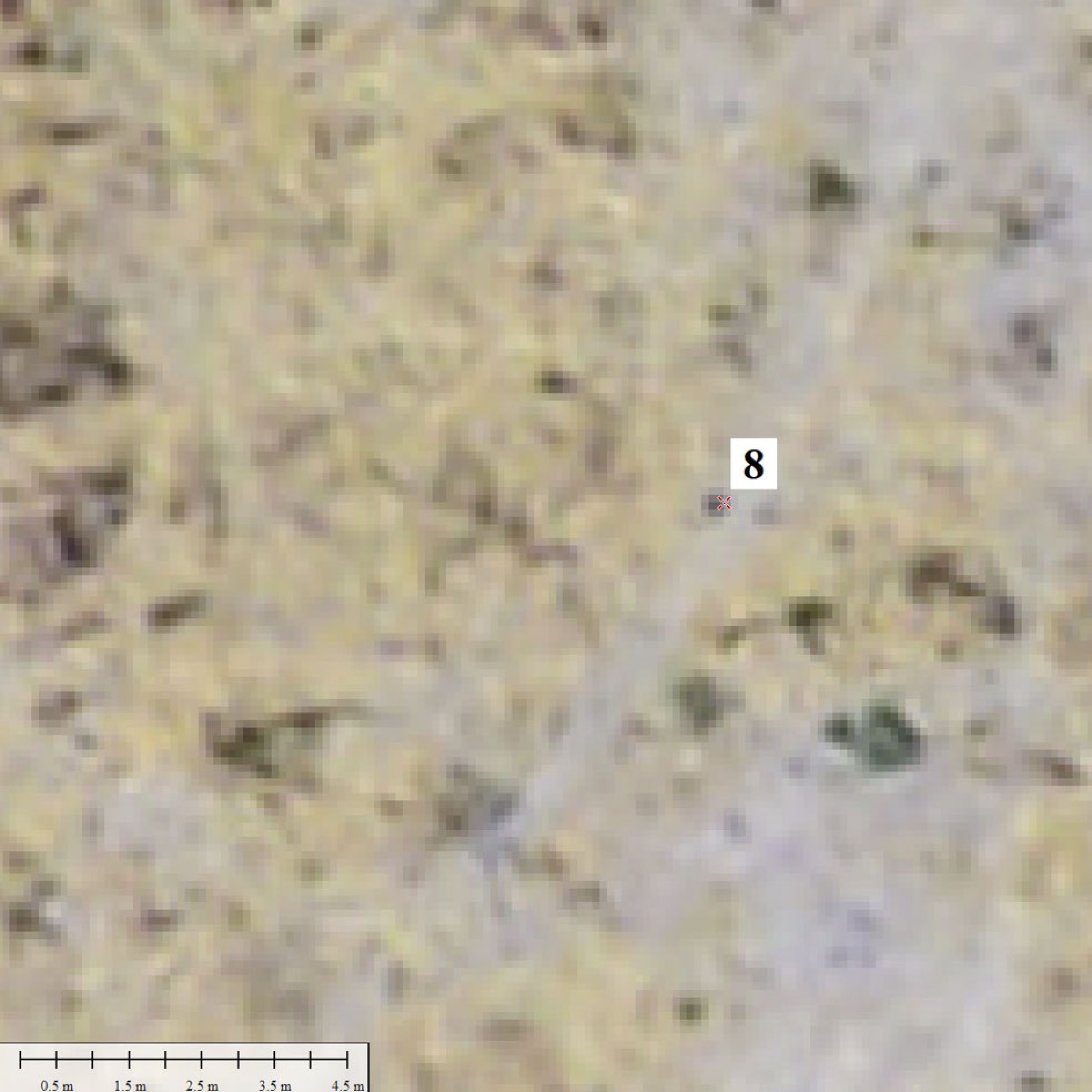
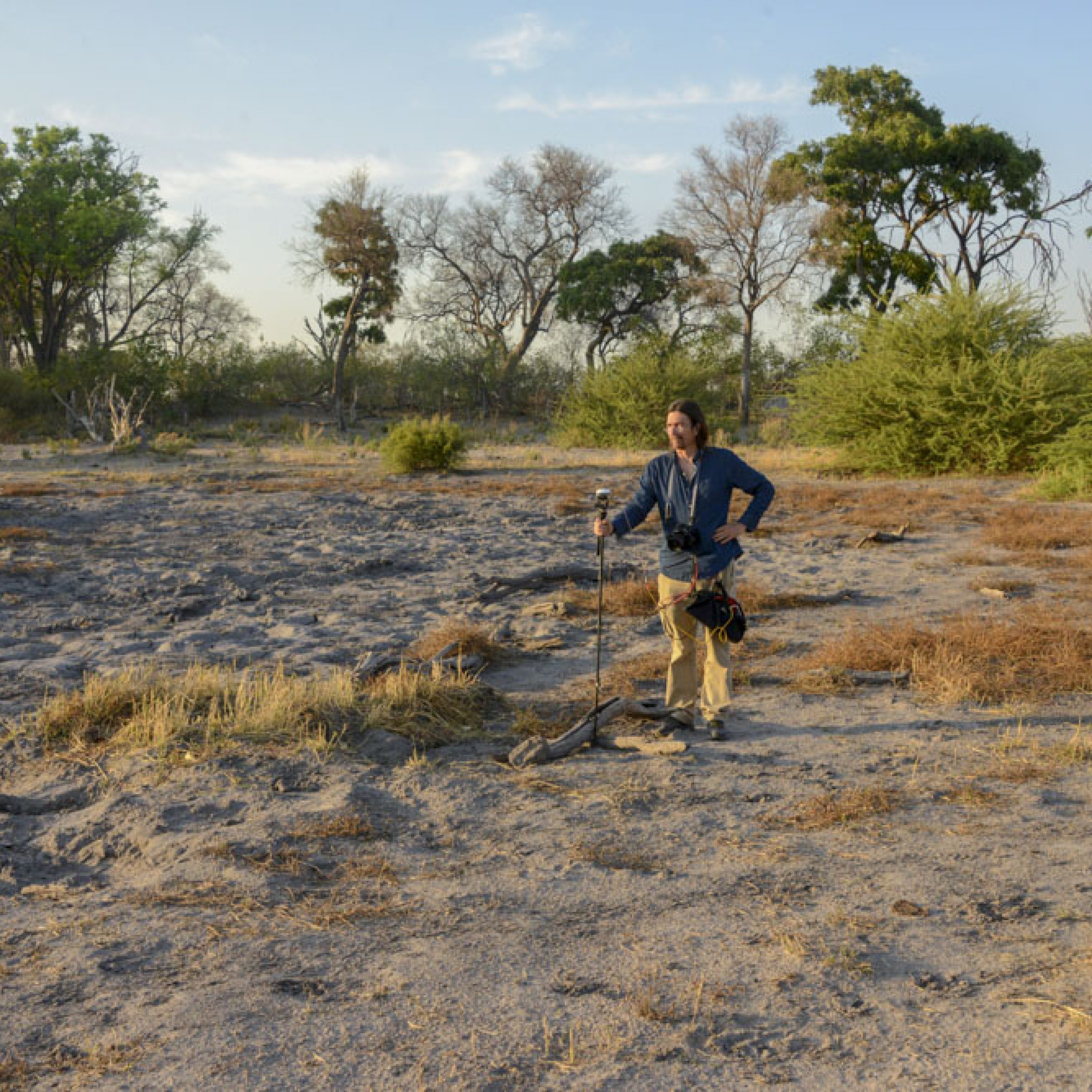
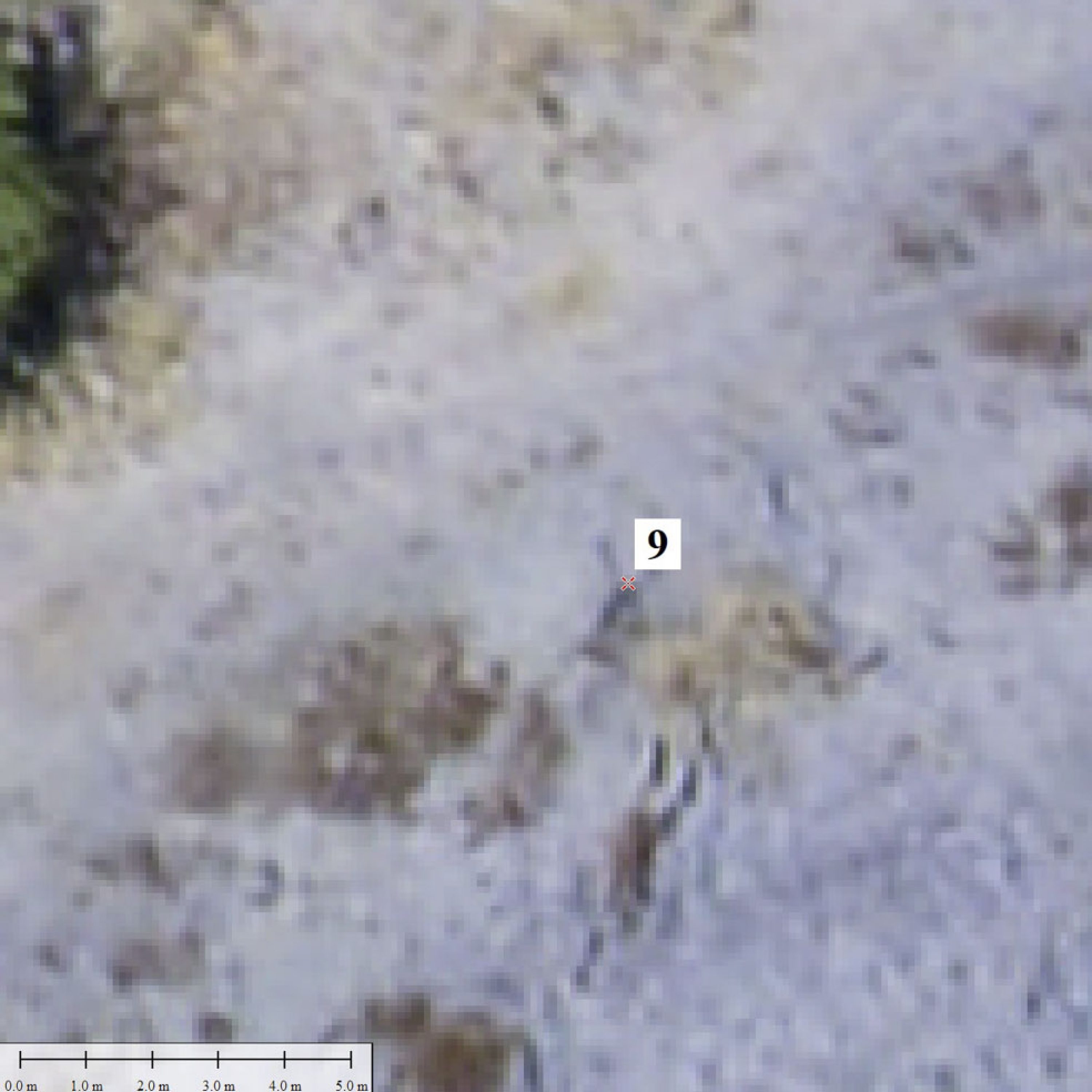
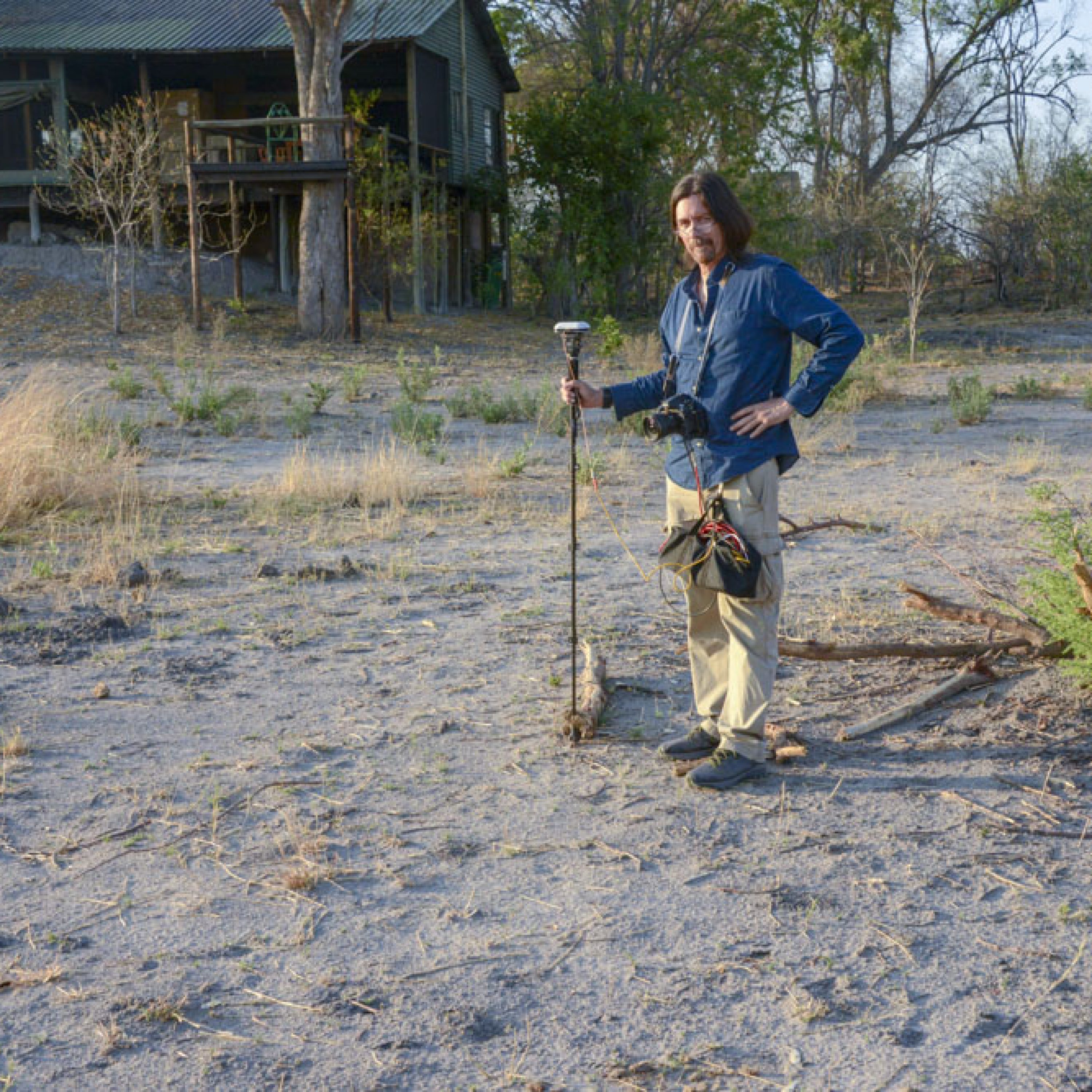
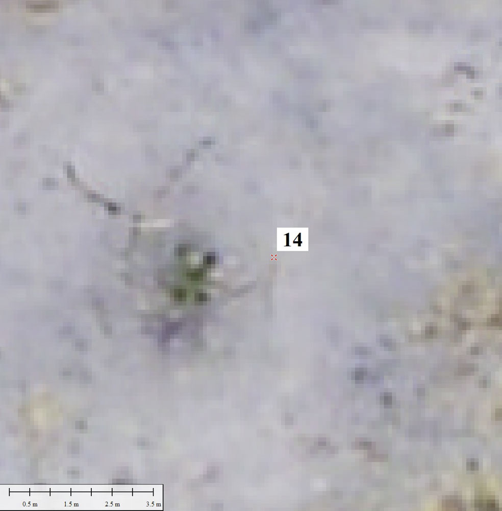
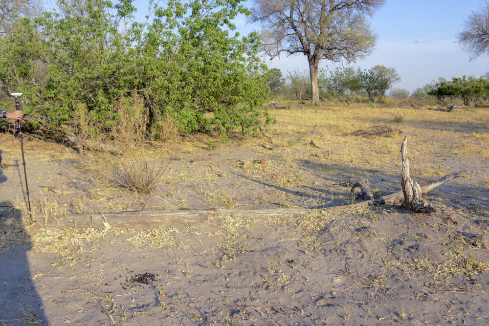
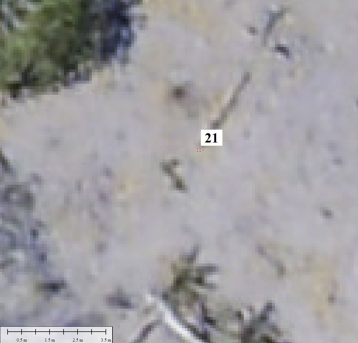
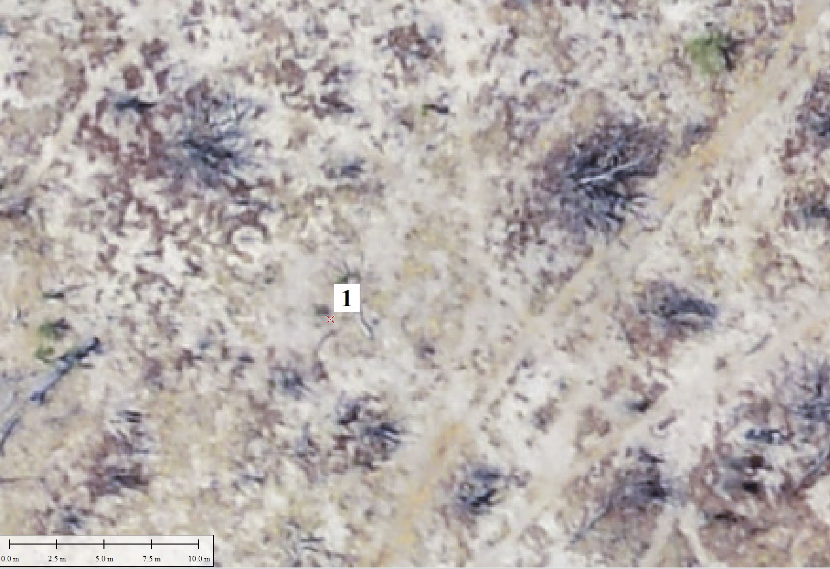
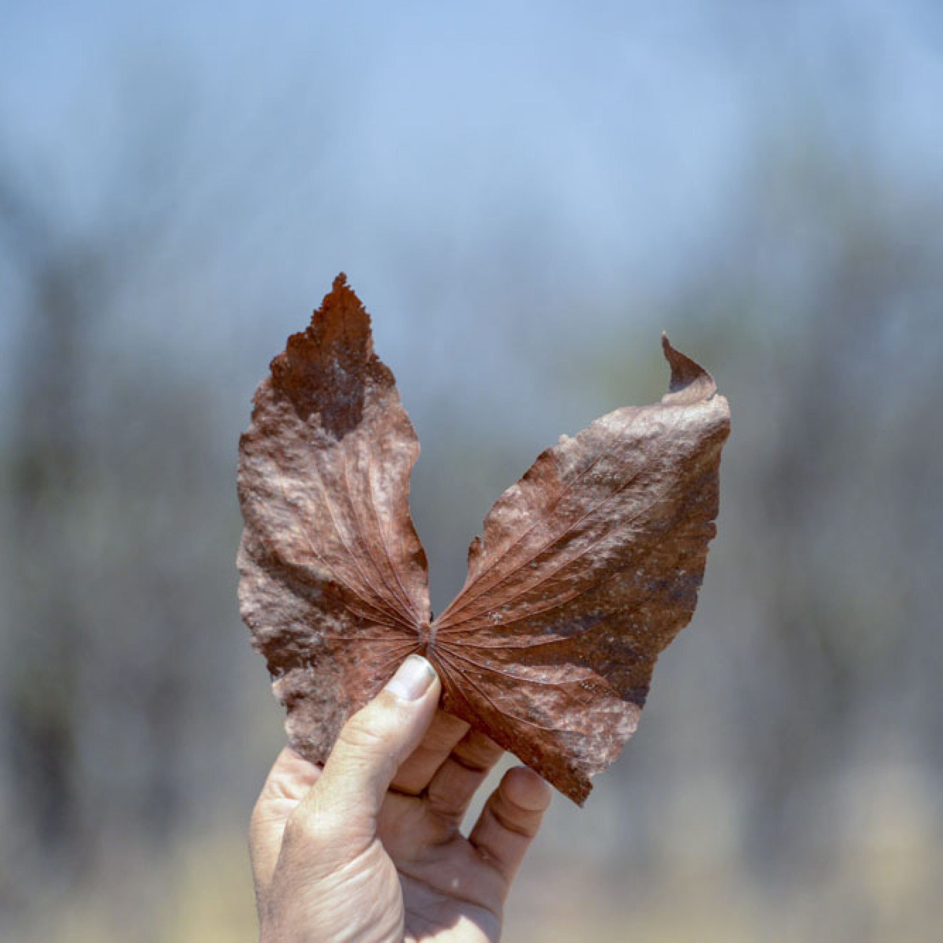
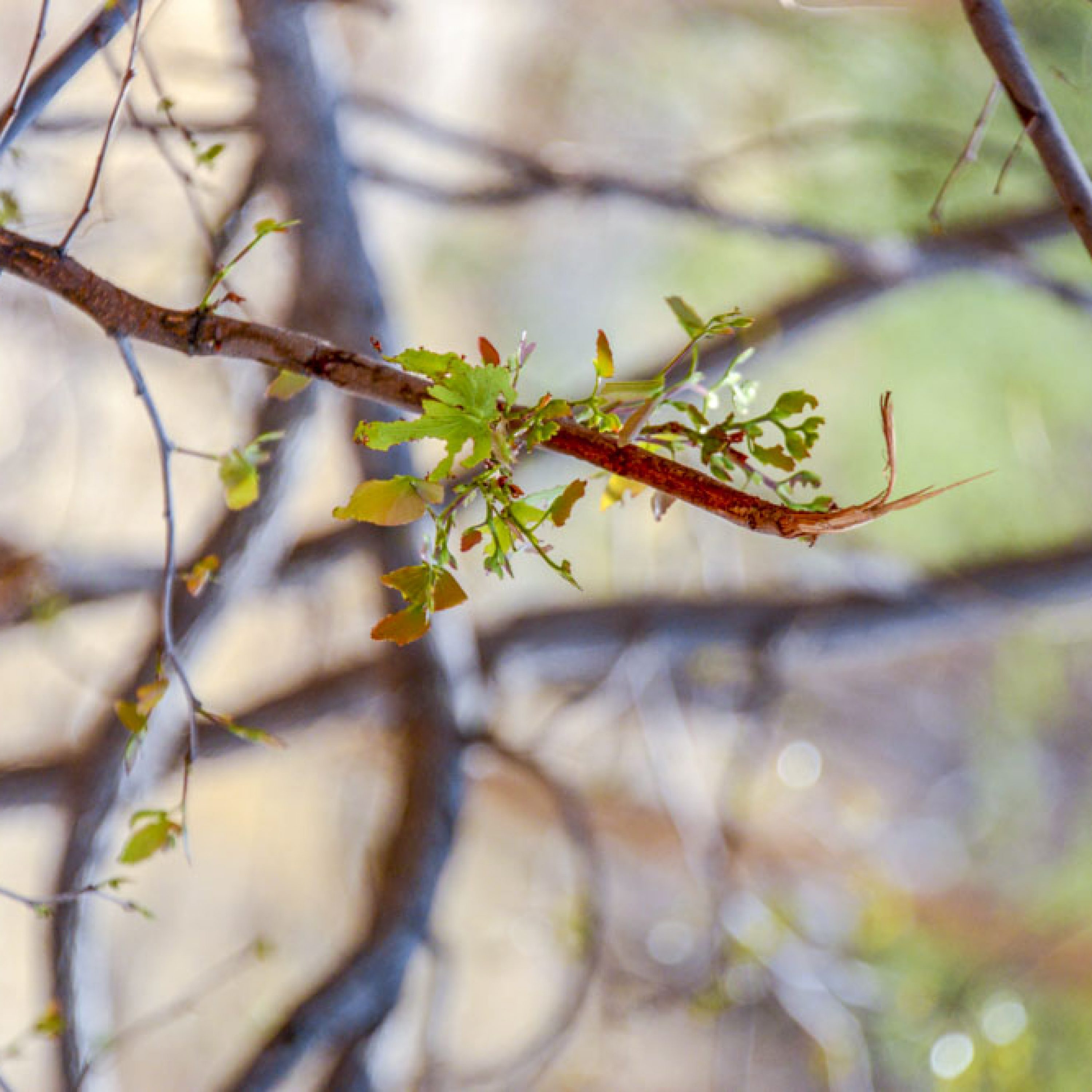
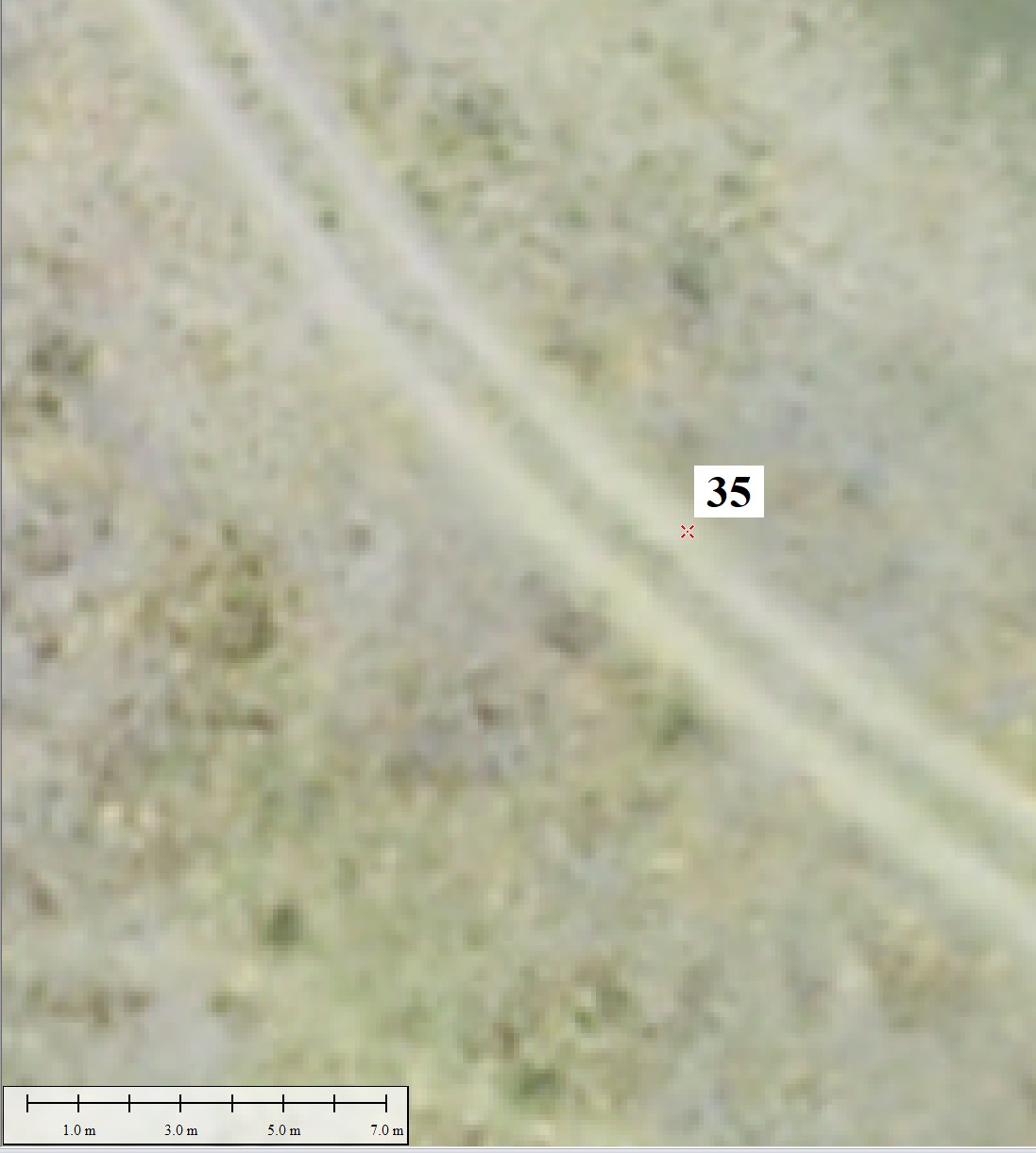
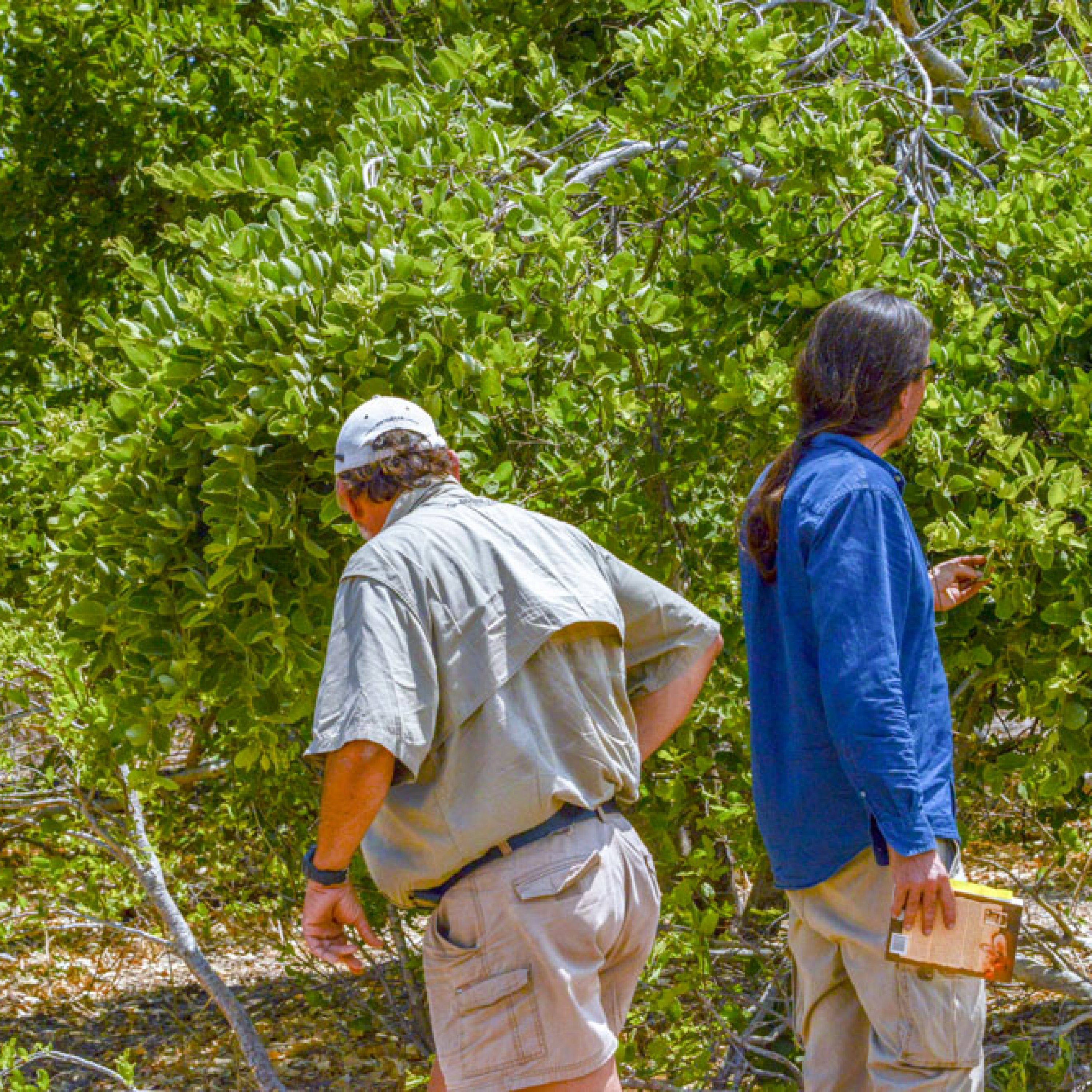
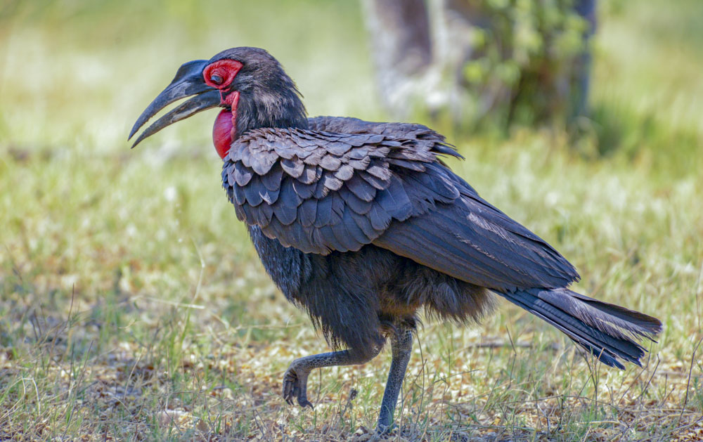
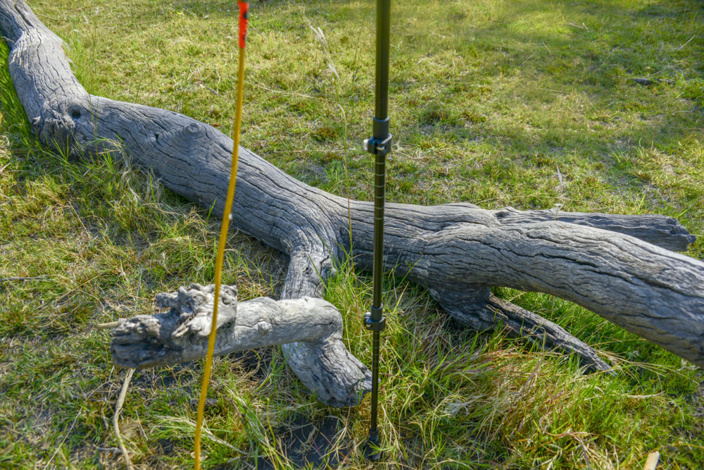
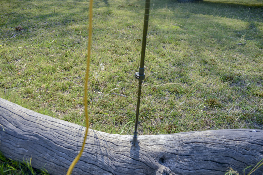
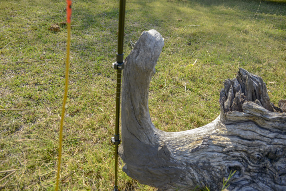
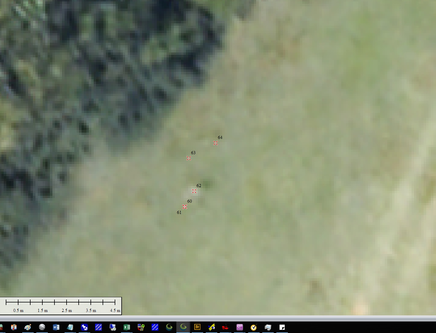
Here are most of the points I measured by walking around CSU camp.That’s Richard’s University vehicle in the lower right. Turner and I slept in the tent to the left of that. The camp managers’ cabin is at the far left.The large green roof is the main offices and garage for CSU camp. This is not a place for tourist, this is the central support unit for those tourist safari camps in the surrounding area. A great bunch of people work here, including John and Francine who helped us tremendously and always with great cheer. We were too busy to meet most of the staff, but it seemed most nights the area in front of the garage turned into a soccer field.One of the challenges in surveying checkpoints is finding natural targets large enough to show up in the airborne images so you can precisely find them in the maps but also that have an elevation that is constant over several pixels so as not to spatially bias the vertical comparison. This termite mound was about as small as could be reliably found in the imagery, but because it is not flat and it is too small to be resolved topographically from the air, the ground measurement is a bit higher than the airborne measurement. See the map view of this spot below.The red crosshair is essentially exactly over the termite mound in the previous image.These logs are not the most ideal for checking elevation measurements at the centimeter level, as the map will average log and soil heights, but great for horizontal comparisons.See here how the red crosshair from the GPS on the monopod fits right within the crossed logs as in the previous image.This log is just barely detectable in the imagery, though this was not clear at the time of measurement. That’s one of issues I hoped to sort out with these tests.The log in the previous photo is just barely detectable here.Big logs like these are easy to find in the imagery, and their partial burial give some confidence that they have not moved in between airborne and ground work.I found no issues with horizontal alignment.John drove us out of CSU to the south to spread out our measurements, but I had some trouble with the rig this first time and also with getting enough satellites. But we got to see some new terrain and learned how much cicadas love stunted mopane forests.You can tell immediately from the fodar orthomosaic that this is a mopane forest by the red leaf litter.The reddish color you can see on the ground in the previous image and all across northern Botswana is caused by these dead mopane leaves. They are very distinctive, as there are no other trees with leaves this shape and I don’t believe any other trees have such a red litter them around them.Notice the end of this mopane branch, this is why they are stunted.We arrived just at the start of the rainy season. Notice how thick these trunks are compared to their height. The mopane have figured out how to throw up new shoots and roots out of their trunks despite intense foraging.Here is the safari vehicle we used to go from CSU camp into the Spillway Block with John. Here I’m surveying one of the tracks. Note that this seldom used track hasn’t fully broken through the vegetative mat; most well-used tracks are incised by 20-30 cm into the sandy or clayey soils.Here is a closeup of the previous photo, showing a smushed termite mound.When I look really closely, I can convince myself I see that dark patch under the red crosshair, but it’s marginal at best. Other clues are needed for this. But it does show up square in the middle of the track for sure.John was very helpful in helping me identify trees.I spent a lot of time reading that excellent book on trees. By the end of the trip, there were probably 20 species I could name without hesitation. Though now, 3 months later, it’s largely a blur, but I think that’s an apple leaf behind me.Turner’s favorite bird — the southern ground hornbill.
After leaving CSU camp, we spent a week or so in the Central Kalahari Game Reserve to gain a better understanding of that ecosystem and its mapping needs. When we returned from there, we spent a few days at Selinda Explorer’s Camp, run by Great Plains Conservation within our Spillway Block. It is an excellent camp with a first-rate staff, and though we were there essentially as tourist they were happy to accommodate our strange photographic requests.
We continued our ecological studies within the Central Kalahari Game Reserve, but a highlight of the trip was visiting Mark and Delia Owen’s camp site where they did their field work described in Cry of the Kalahari.The view from our first tent at Selinda Explorer’s Camp.We stayed in a double-wide the first night. Upscale.It only appears like a tent…
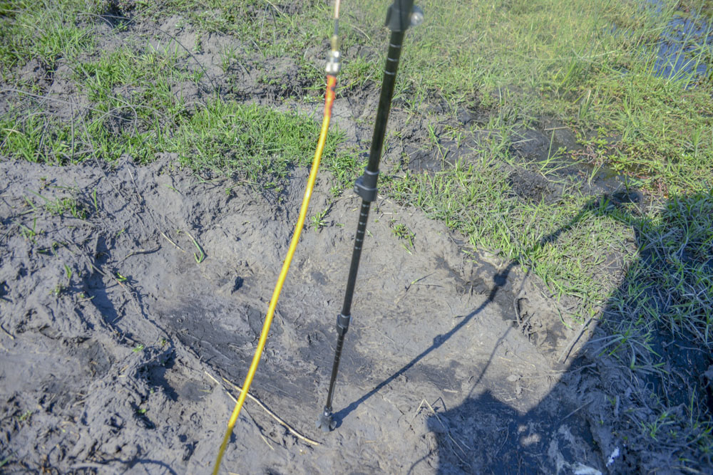
Next I compare our ground tracks measured with precise GPS while driving in our safari vehicles. Here at various times throughout the day I used the airborne system as we went on game drives. The antenna was located above the left-front wheel well. I couldn’t ask for a better correspondence between the ground and the airborne data based on these tests.
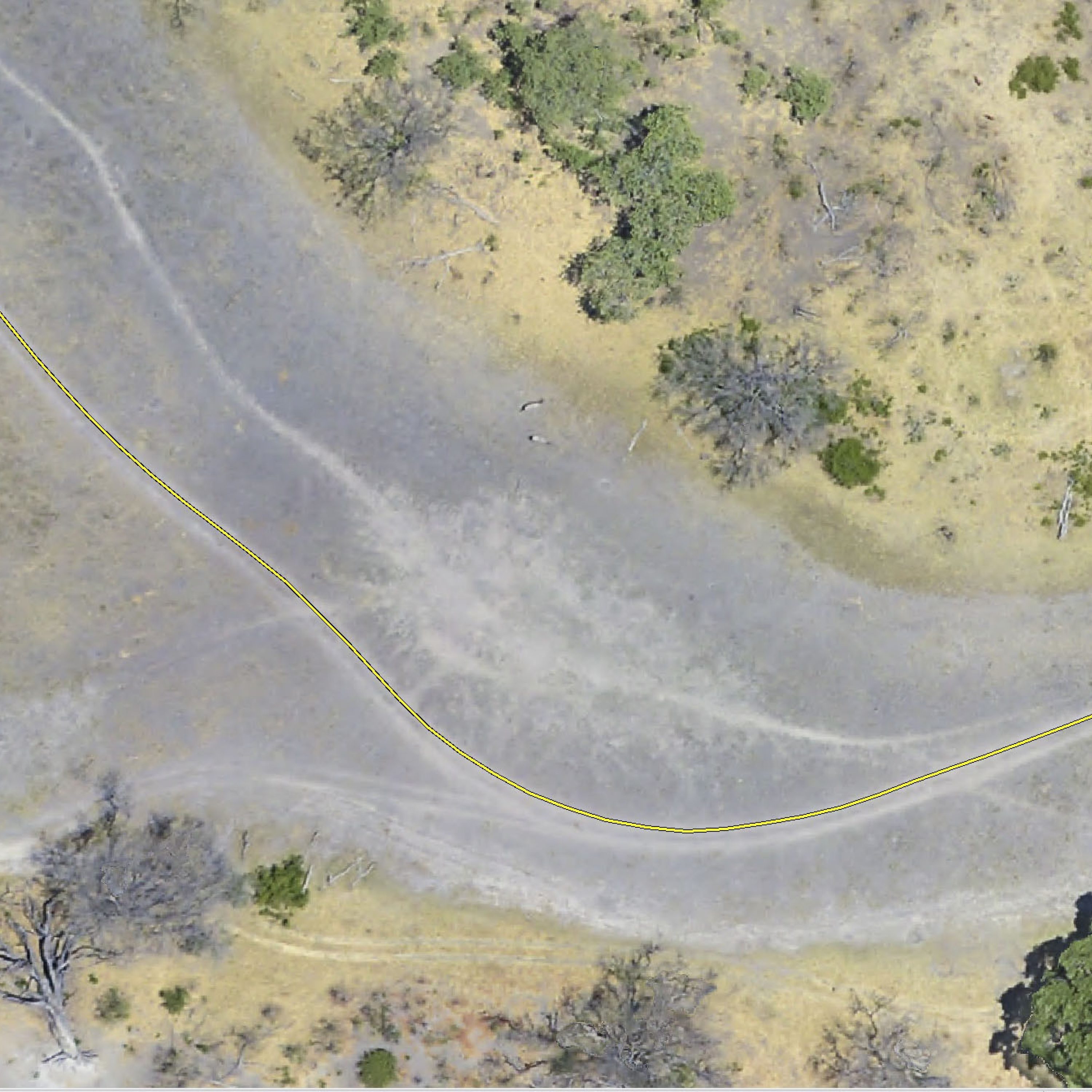
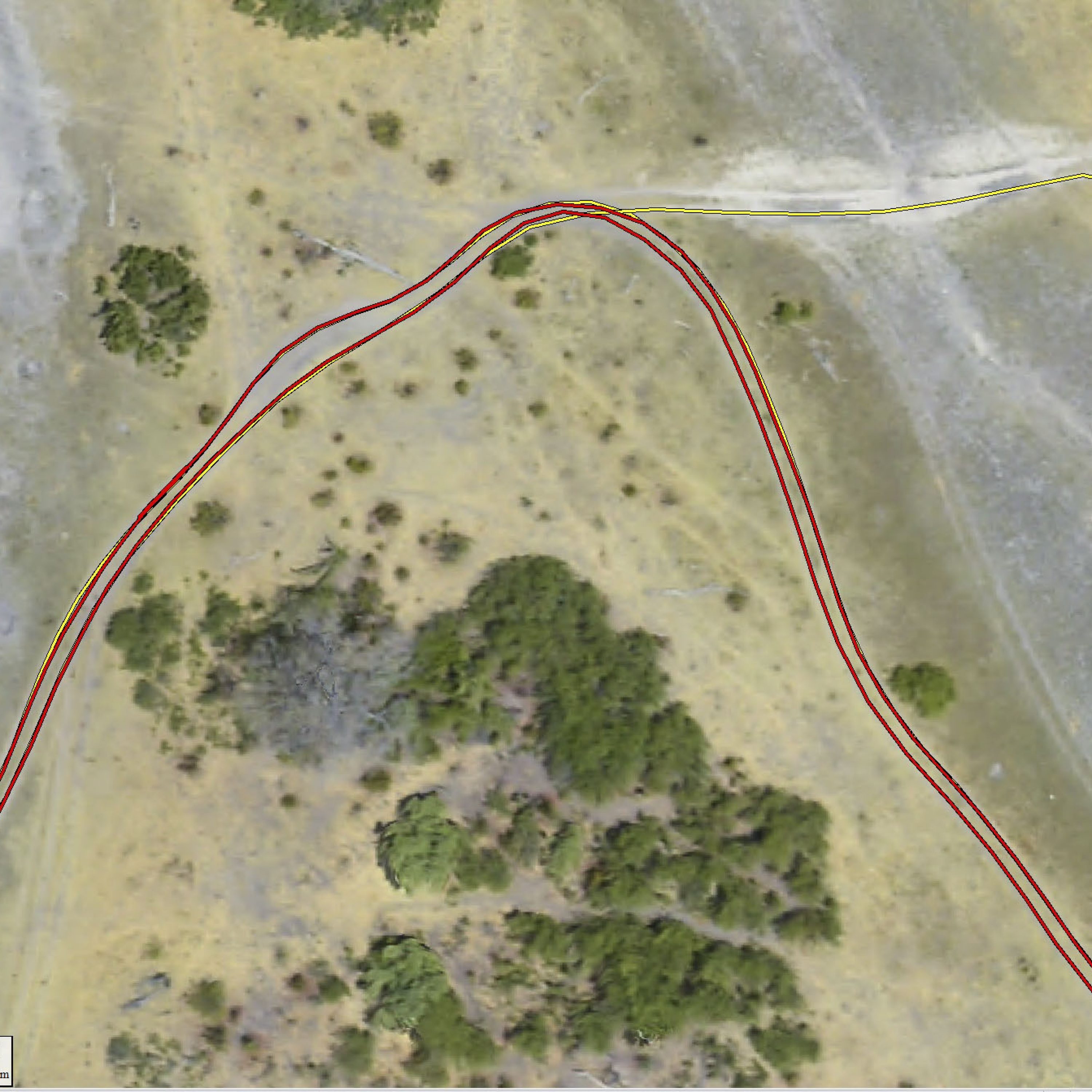
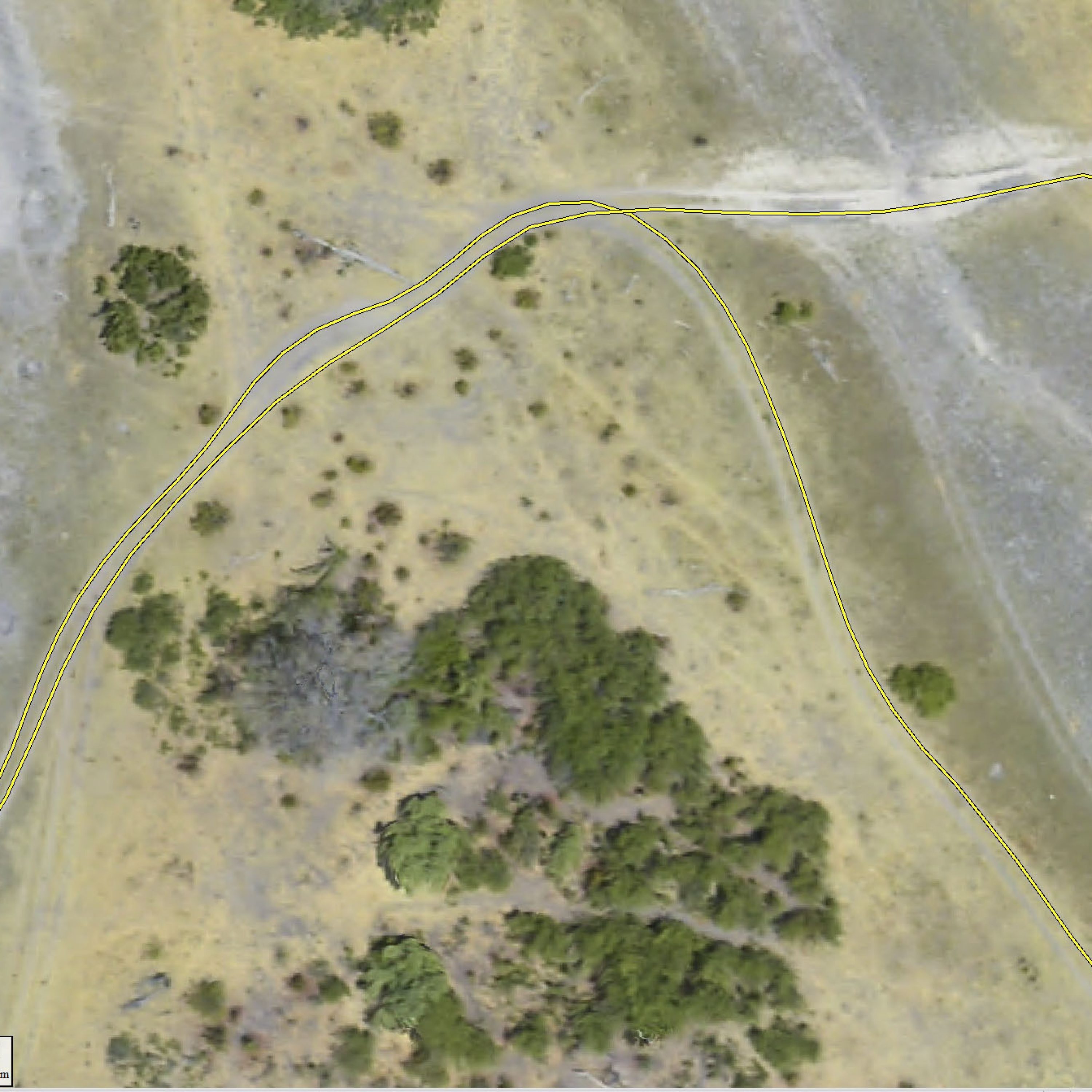
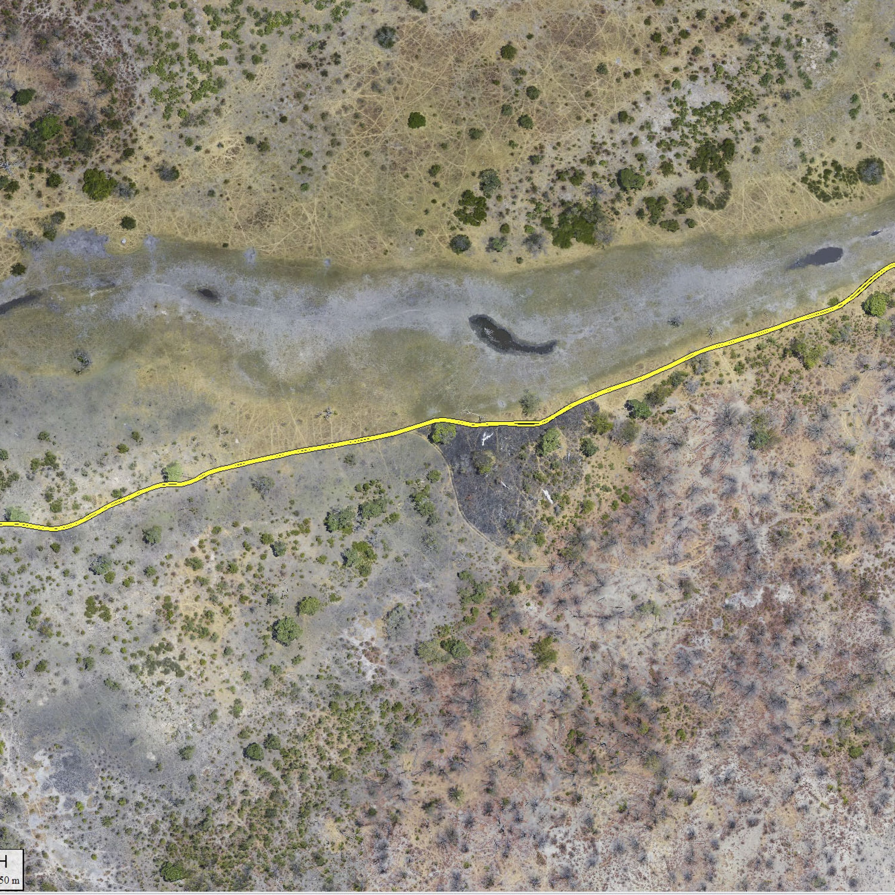
The yellow line is our GPS track from Selinda Explorer’s Camp, as measured with a dual-frequency receiver, processed in PPK against my own base station at camp, so the accuracy should be good to a few centimeters when trees are not blocking the sky view. The antenna was over the left-front wheel well, so here you can tell we were driving from left to right, as the yellow line is directly over the left of the two-tracks incised by the safari vehicles.That in and of itself is a great indication of the horizontal accuracy of the data, as well as mutual verification of the field techniques.
Here we have driven in both directions on this track, such that the antenna was directly over one or the other rut, depending on direction of travel.
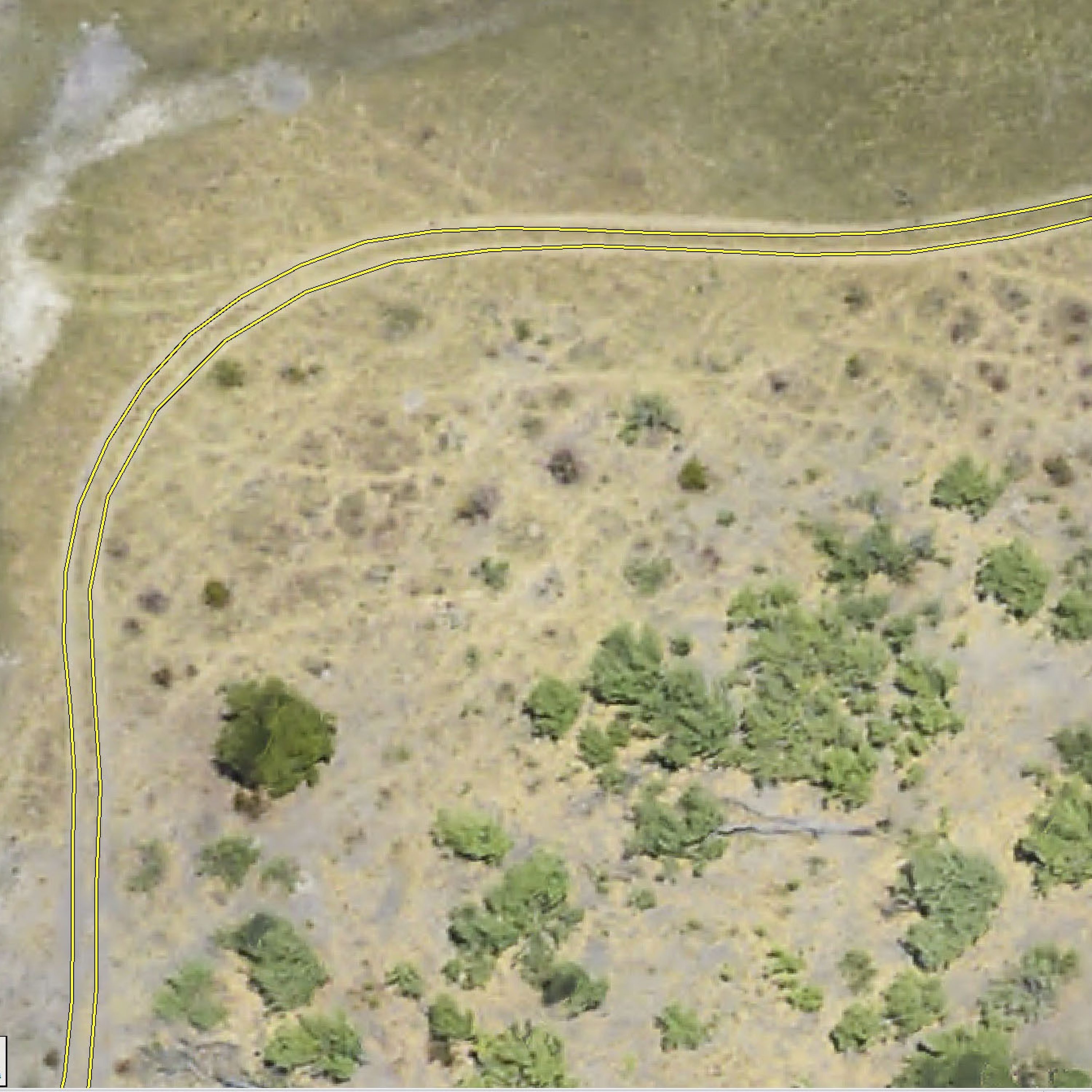
Here several sets of tracks overlap on different days (color) in one or both directions. The antenna was not placed on the vehicle in the exact same location on both days, but in any case the tracks are often within a few centimeters. In driving in one direction on both days, you can see by the wide-spacing in lines we veered to avoid some obstacle, but only going in one direction.
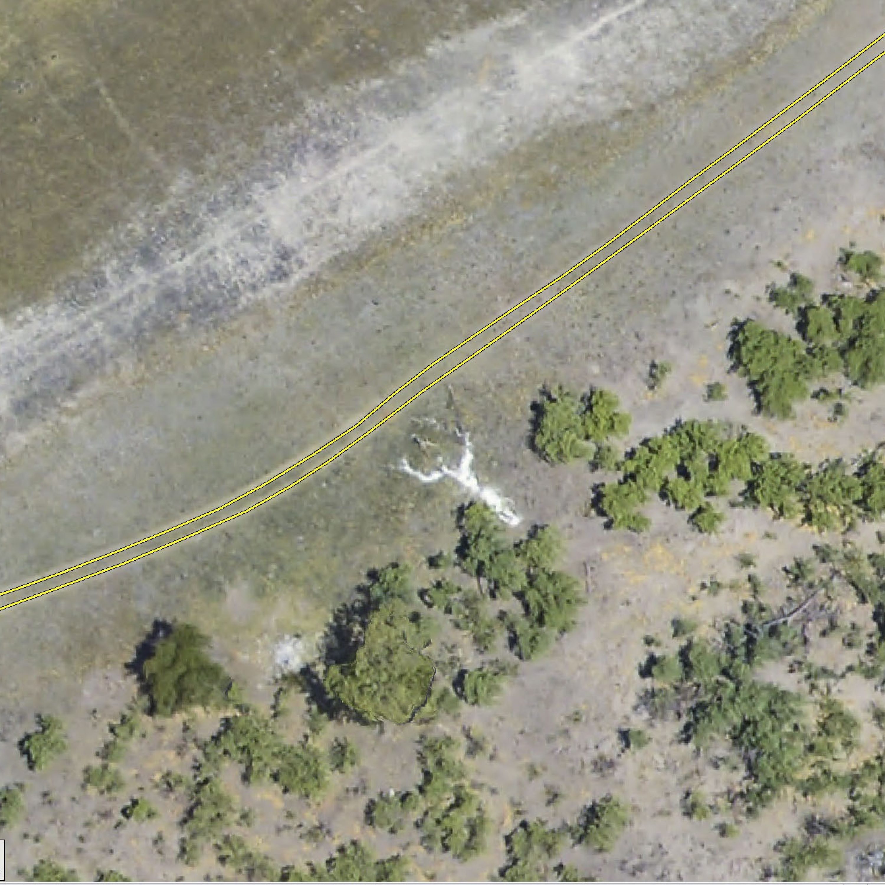
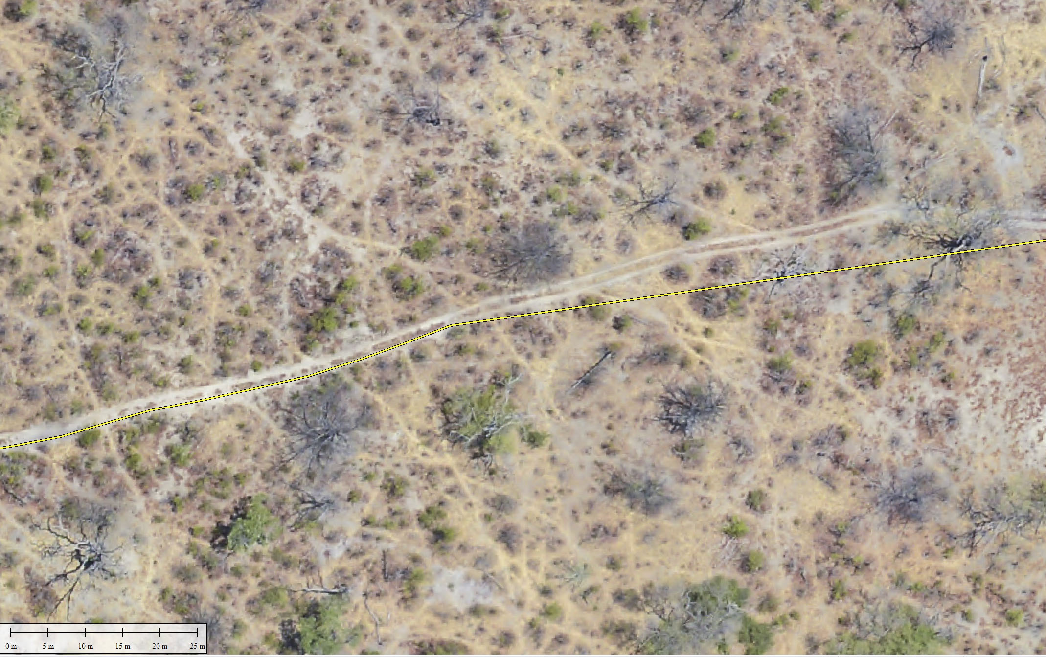
We drove past this burnt leadwood tree twice. These leadwoods are appropriately named, they are really dense and will burn for months and maybe years, leaving their ashen tombstone behind. Because their high contrast and flatness against the ground, they would make great GPS targets for ground control!Driving through brush and under canopies can lead to loss of accuracy, as seen here, where the yellow track veers from the image’s vehicle track.
Even when the GPS fix holds under a tree, comparisons of the vertical dimension between the ground track and map will be skewed because the ground vehicle is measuring topography under the tree and the airborne map is measuring topography of the tree canopy.
Here is a closeup of the ground track over the topography. The vehicle tracks are incised into the ground by 10-30 cm or so. They are clearly resolved in topography, but skewed a bit upwards as they are only 20-30 cm wide, so there is a bit of spatial bias caused by the higher edges of the tracks, as the elevation of the edge and the rut get averaged together a bit. But as best I could determine it, the mean vertical misfit was only a few centimeters.
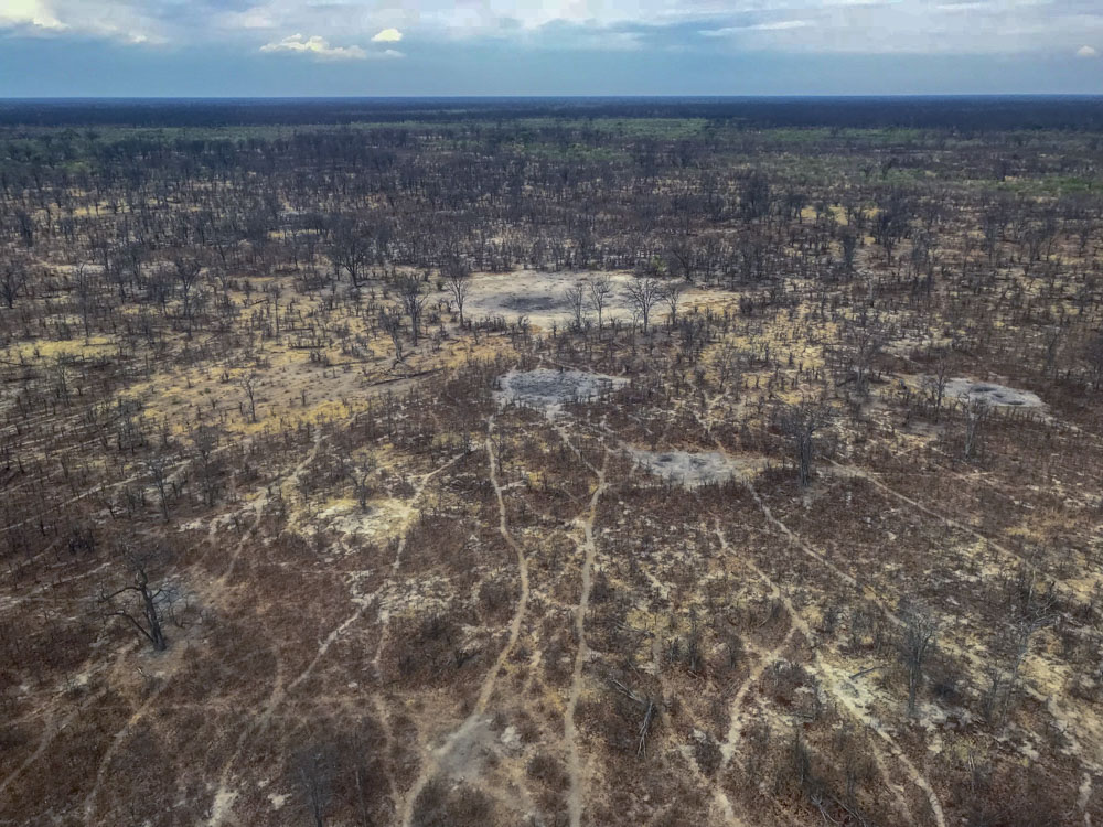
Here our tracks transition across into a mopane woodland which has not yet leafed out, though last year’s red leaves are still visible on the ground at lower-right. At center is a burned scar, perhaps started by lightening, which was apparently contained by the vehicle tracks in the sandy soil the left and the siltier and probably wetter soil of the mopane forest to the right.
I really love these leadwoods, a crop of the previous image. They are spectacular looking trees in general with really cool seed pods, but the ghostly outlines they leave behind are such interesting features on the landscape. These will also make great alignment targets for time-series of fodar maps like this.
In total we made over 23,000 measurements using this driving method. I filtered these down to about 8,000 by quality statistics from the GPS processing software so that I was mostly only using ones unaffected by poor sky view in the trees. I then used the middle 95% of those to calculate the range of vertical misfit of +/-13 cm for 11,851 points, about a mean of several centimeters (discrepancies in antenna heights prevent an exact value). Considering the suspension travel on the vehicle is over +/- 30 cm, the spatial biasing caused by the narrow, incised tracks, and the fact that some percentage of these points were still under a tree canopy (as in the last image at left), this is an amazing result and totally in line with what we’ve seen in dozens of other projects. Considering the horizontal accuracy shown above is nearly perfect, I have no reason to suspect the vertical accuracy is any worse, and my best guesses at antenna heights show it to be within centimeters.
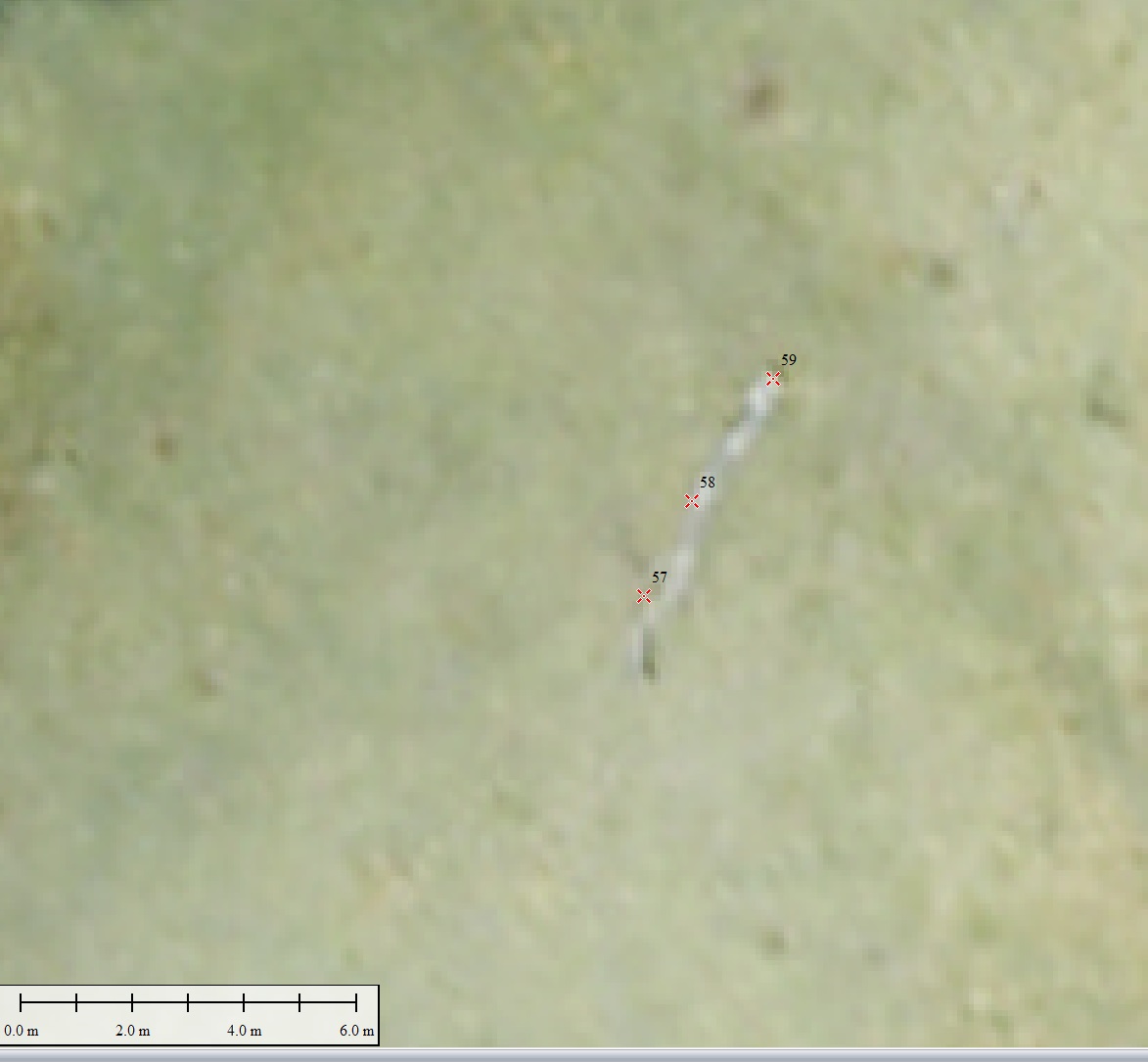
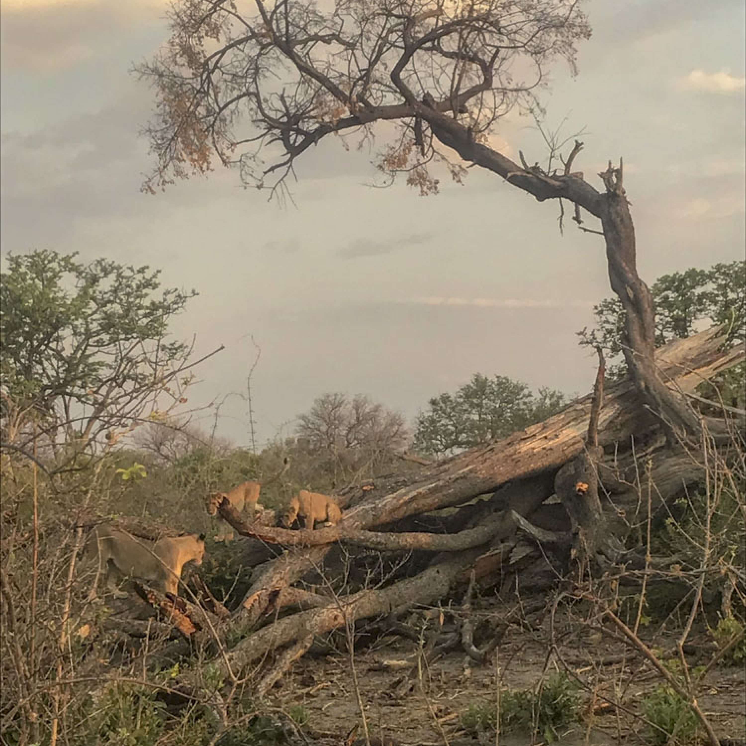
Here are a few more walking points we collected during a breakfast break from Selinda Explorer’s Camp.This log showed up nicely in the fodar orthoimage and the three GPS points (shown below) plot perfectly on top of it. Recall that no ground control was used to create these airborne maps, they just magically appear in the right place due to the techniques we use.Most of the branches I found in this cluster were too small in the imagery to be satisfying, but this big scrape showed up well enough, below.With enough scraping, eventually this pothole will turn into a pan.Here you can see the magnetic GPS antenna over the left wheel well, opposite of the side that our excellent guide Oats is on. I could get used to this type of field work…We spent much of our time in Selinda Explorer’s Camp following around a pride of lines. They spent a lot of time sitting in the shade and playing in woods, woods impacted by elephants in a variety of ways.
We got to know many of the pride as individuals during our time there, and spent much of our time about this close to them.
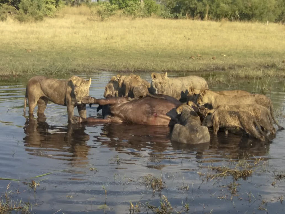
After 3 days of watching them hunt unsuccessfully, they finally tackled this buffalo on our last day there.
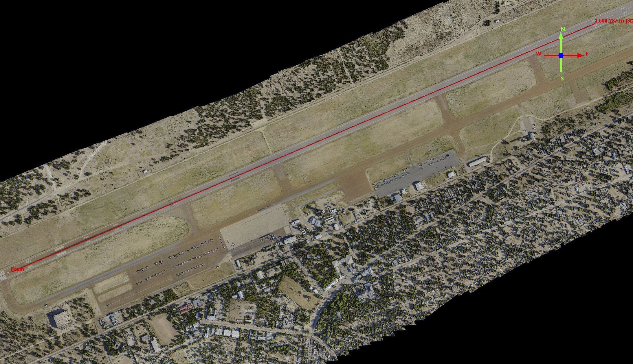
We also have overlapping and independently-made maps at several locations, which gives us another opportunity to assess accuracy. Here I show several of those analyses. The first comparisons are of the Maun airport and the Boro River not far from it. Note that these maps were made not for production but for system shakedowns, so they all have some wonkiness. For example, on our first flight the camera nearly fell off because I had forgotten to tighten the clamp sufficiently (it was backed up though, so it would not really have fallen off) and between Joe learning to hold a very tight heading while ATC was pushing us around, line spacing suffered from optimal. Despite these challenges, the comparisons were outstanding, so I expect the real data to be even better.
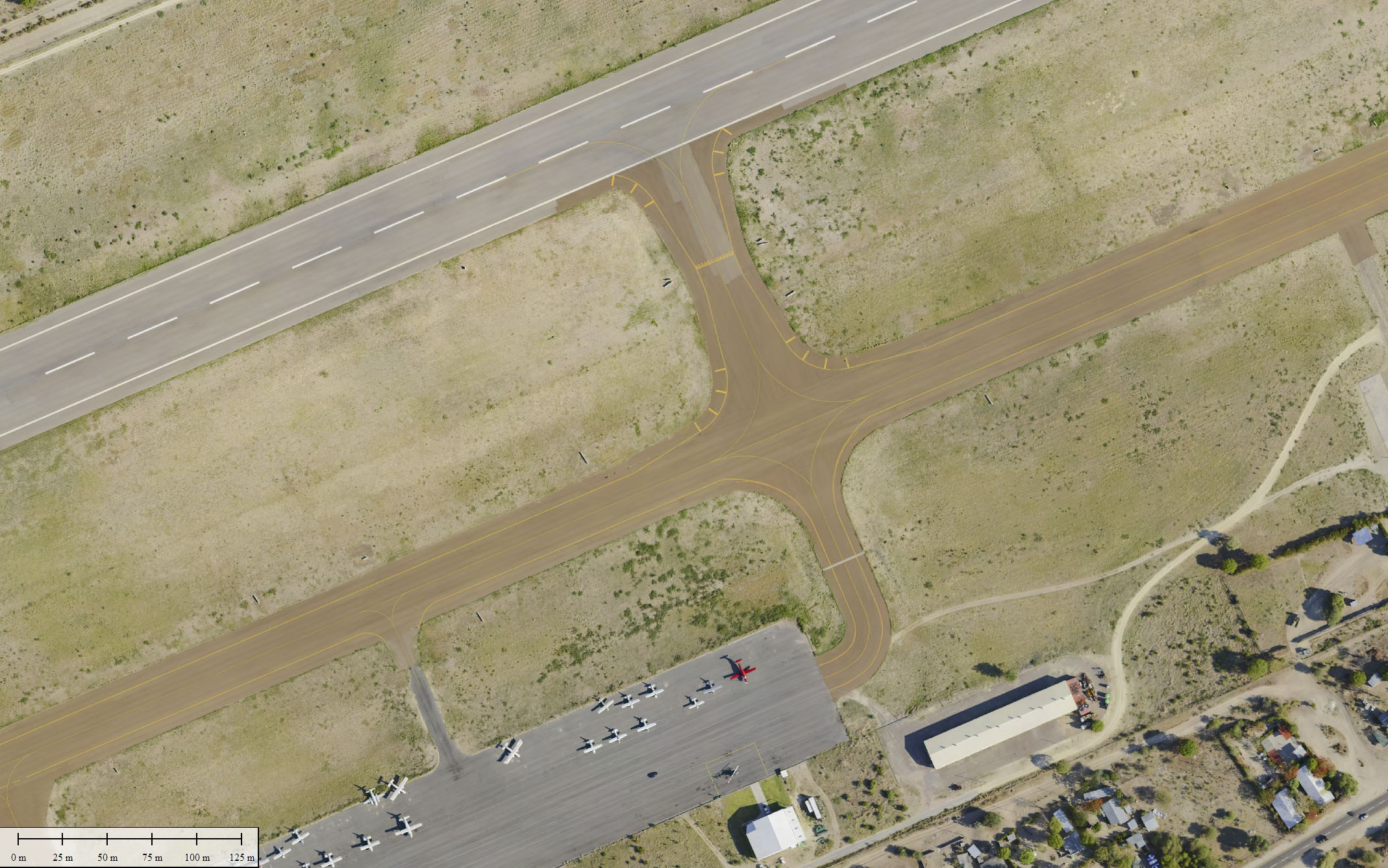
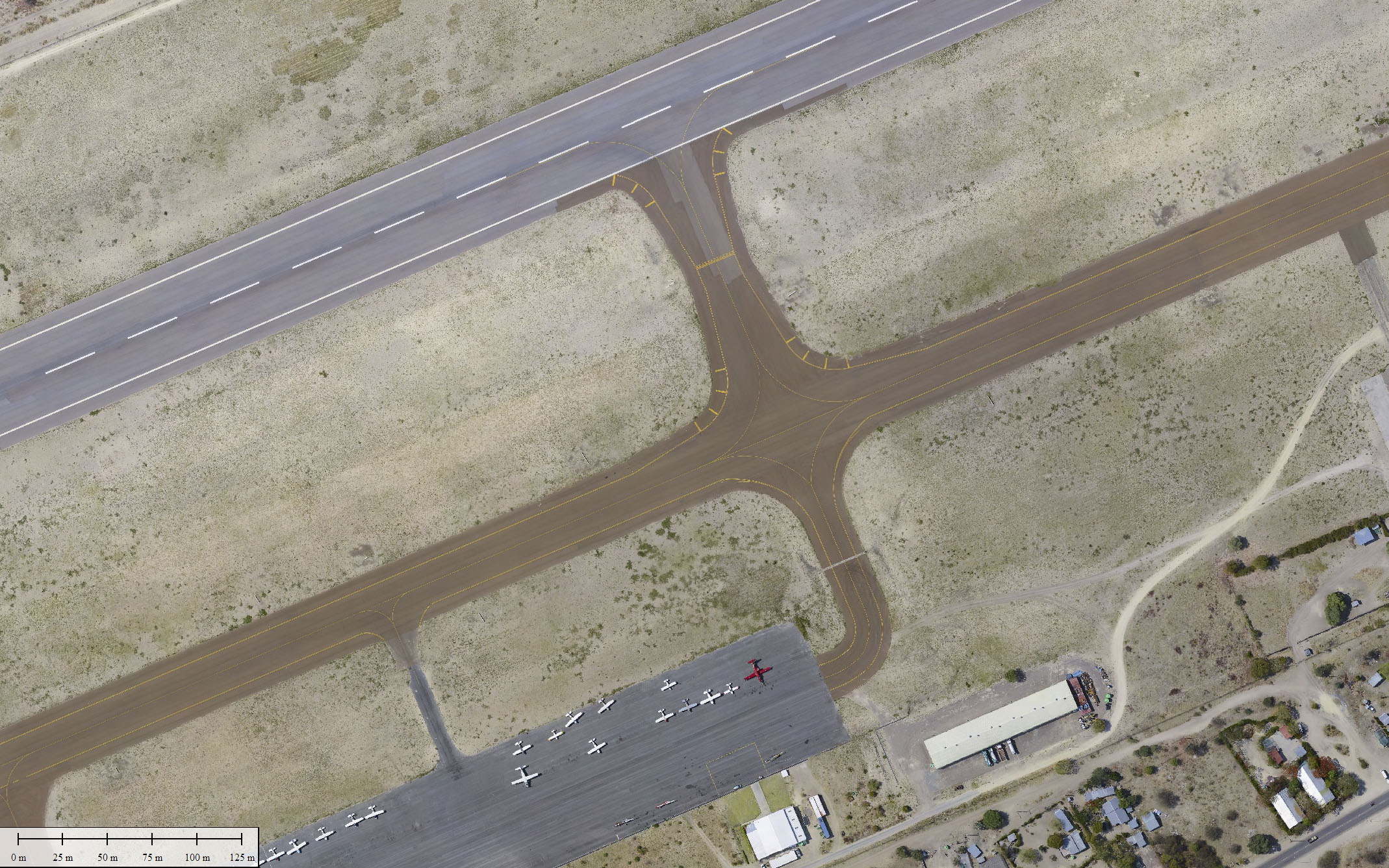
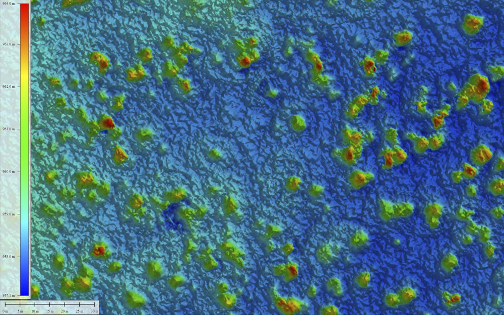
Here is an example of the horizontal precision between 2017 and 2018 fodar maps of the Maun aiport. The shadows can make things confusing, stick to looking at the runway markings.
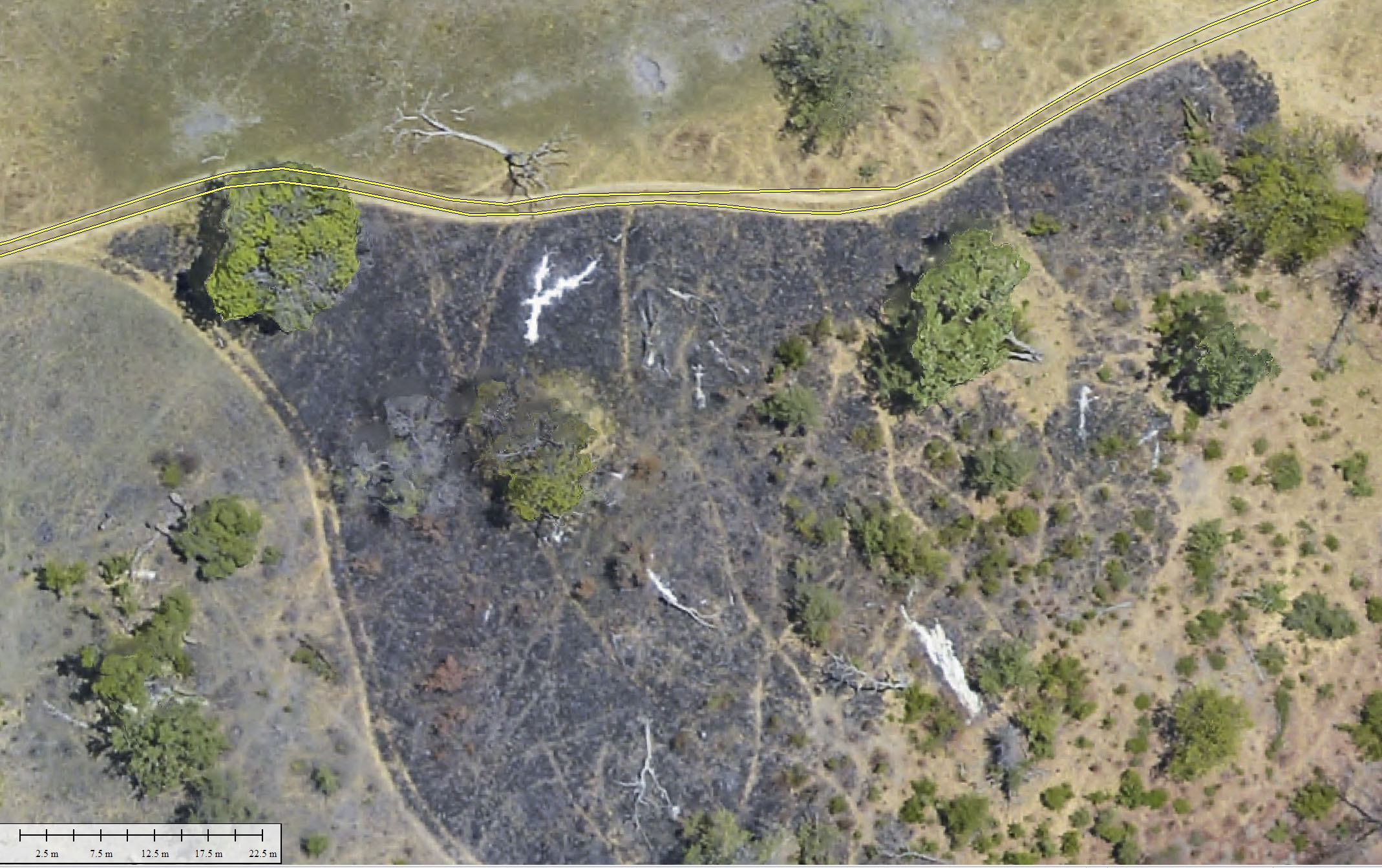
I’ve heard Maun described several times as a ‘drinking town with a safari problem’. The Tandurei restaurant, shown here with the courtyard with the red plane in it, is one of the main places local pilots go to escape their problems. Note that several trees have been removed near the road; I’ll revisit these later as an example of detecting elephant browse. Note also that the differences in shadows can play tricks with your mind, so when assessing horizontal precision here focus on road stripes at first.
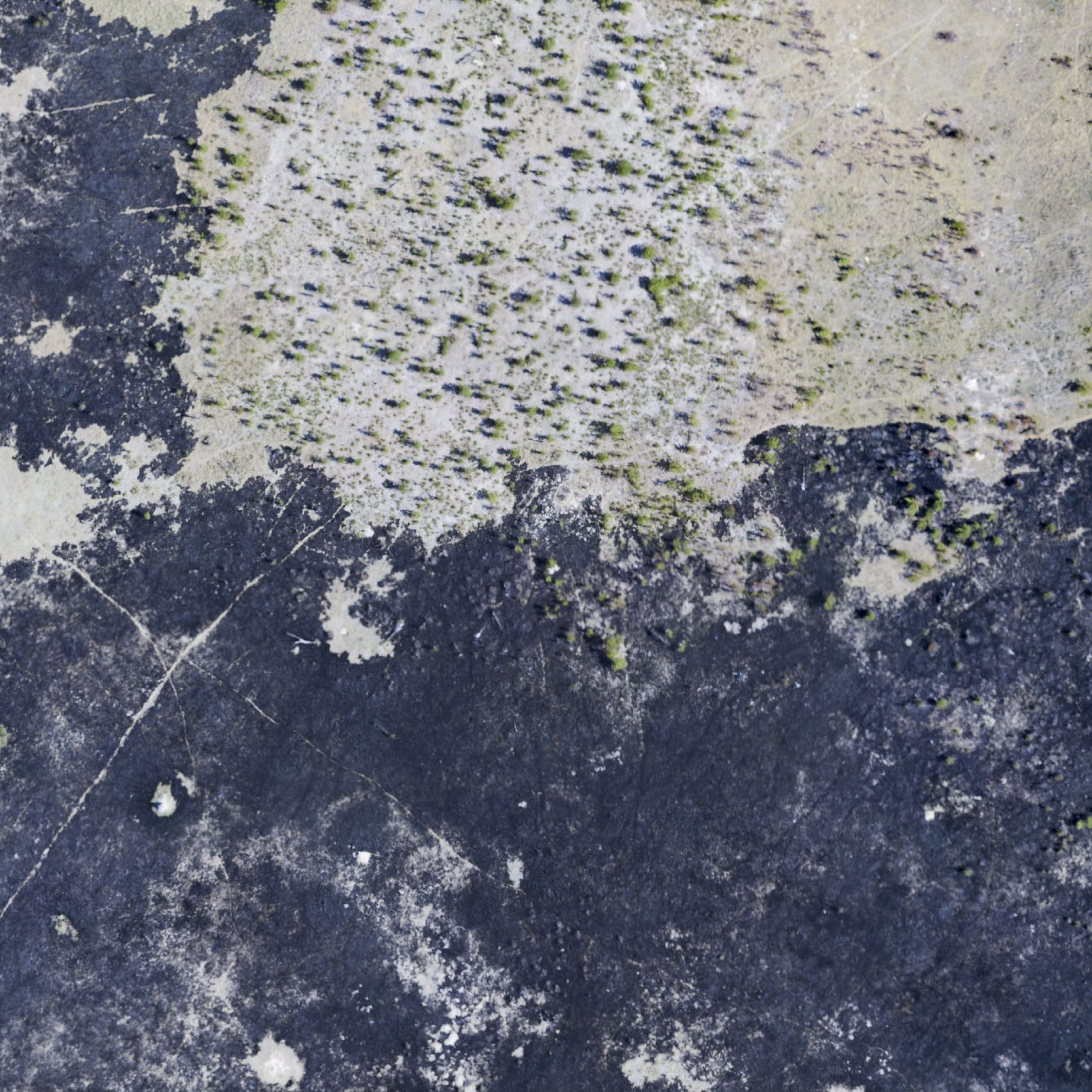
Here is are a few example tests of spatial alignment between 2017 and 2018 fodar maps made along the Boro River, not far from Maun. In 2017, we walked across that fresh burn scar. The grasses here have adapted to quickly regrow after fire, as their roots remain largely unaffected by burning or grazing. My suspicion is also that the spatial extent of the burn says something about the change in soils and soil moisture at the boundary and could be a useful tool in mapping such soils.
The spatial alignment is spectacular, especially considering the hokeyness of how we collected these shakedown data. Not also that image clarity improved in 2018 due some subtle changes in rigging.
Though precision is different than accuracy, in the tests above they are essentially the same. In these studies and all others, when I map the same locations multiple times, they plot in the same locations to within a pixel or two. There is no way the data can be so precise without also being that accurate. Unlike the canonical textbook model of arrows being shot at a bullseye, in the realworld we have no bullseyes so we have to use repeatibility as the test for truth, just as we do for GPS measurements on the ground. And given the close correspondence between our ground-based GPS measurements (shown previously), we have no reason to believe that horizontal accuracy here is anything other than 1-2 pixels.
The airport is also probably our best location for measuring vertical precision and accuracy, largely because we can eliminate the issues of vegetation and vegetative growth. Having determined that horizontal accuracy is only a pixel or two, we can have faith that vertical comparisons here are meaningful.
The color image shows the difference in elevation measured by fodar in 2017 and 2018, with colors stretched over +/- 50 cm. So the yellow-greens that cover most of the airport are very small differences, 10-20 cm. Presumably nothing has changed here, so the differences would be zero if my data were perfect. The large changes in color at the edges are increased noise, but this is expected as this is edge data with insufficient photo overlap– in a real project I ensure that the edge data are not inside the area of interest by acquiring extra lines.
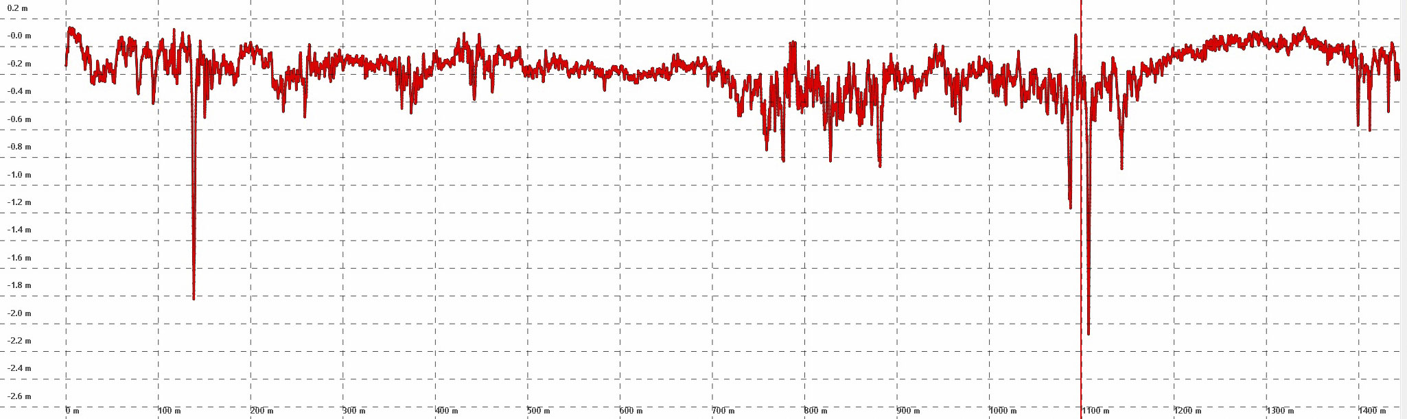
Here you can see the difference in measured elevations along 3 km of the runway, seen as the red line in the previous image pair. That’s n=46,232 points with 95% of points within +/- 21 cm, or a standard deviation of ~10 cm. This is on par with every previous fodar study, though on the high end of error. Regardless, considering there was no ground control involved and we did this within 24 hours of landing after having traveled for nearly 60 hours and with a new pilot, it’s quite an outstanding result I think.Here I’m ignoring the mean difference as I’m not using this as a test of accuracy, due to several confounding factors (one of which is not having any ground truth here), so I manually shifted one of the DEMs to near zero mean. And for all we know without further measurements, some of this variation is likely real, causing by swelling or subsidence of the runway on the order of centimeters.
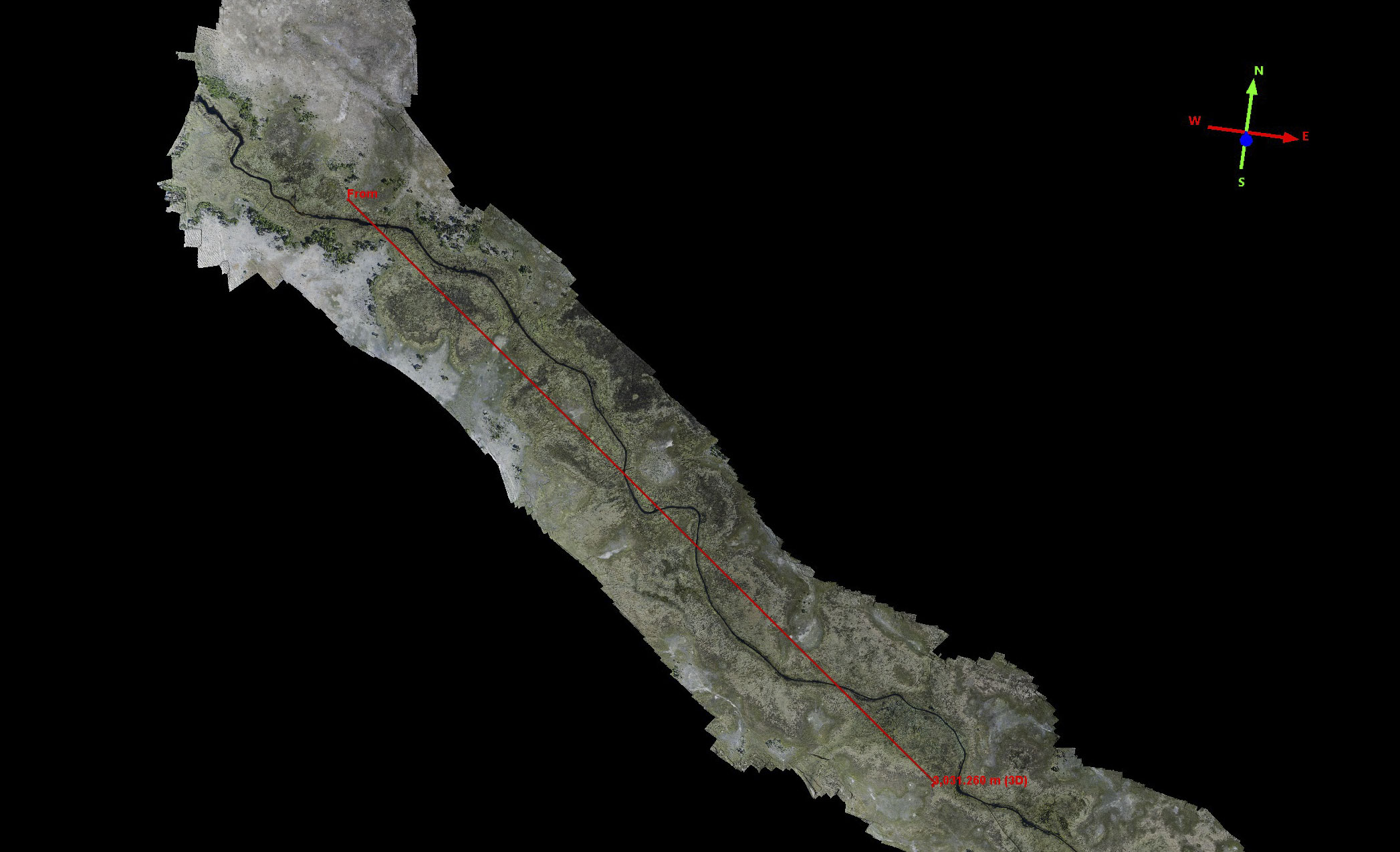
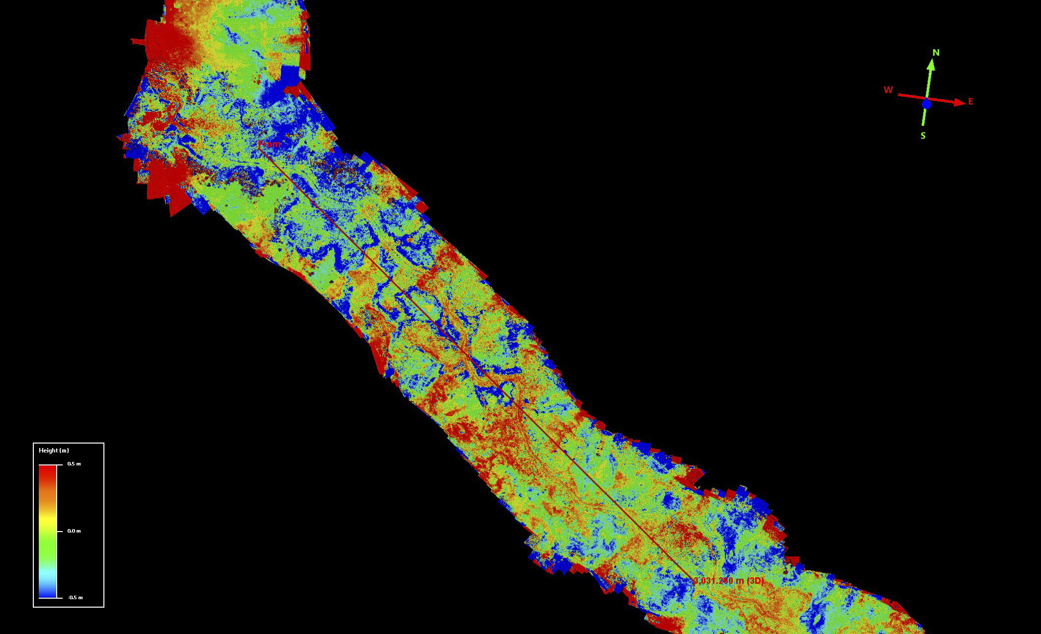
NG18B is the only location we mapped twice in 2018. The second time we flew part of the transect at a lower elevation to test how this would improve our elephant studies (described later). The transect were processed independently so make a great comparison test in many respects, though the results are conservative given the low lines were done ad hoc and not to normal standards.
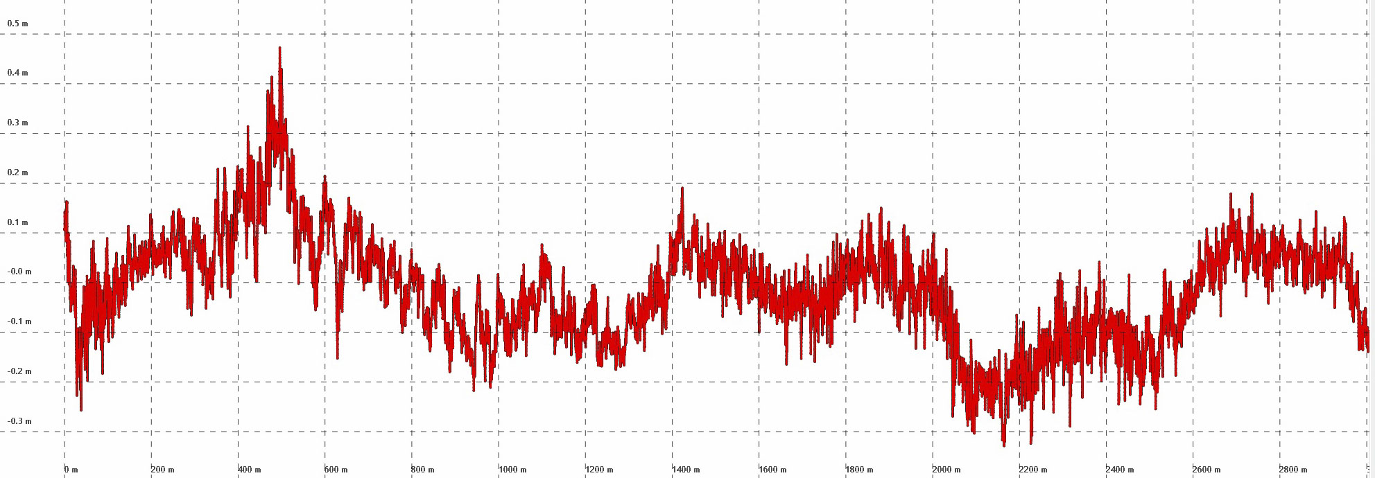
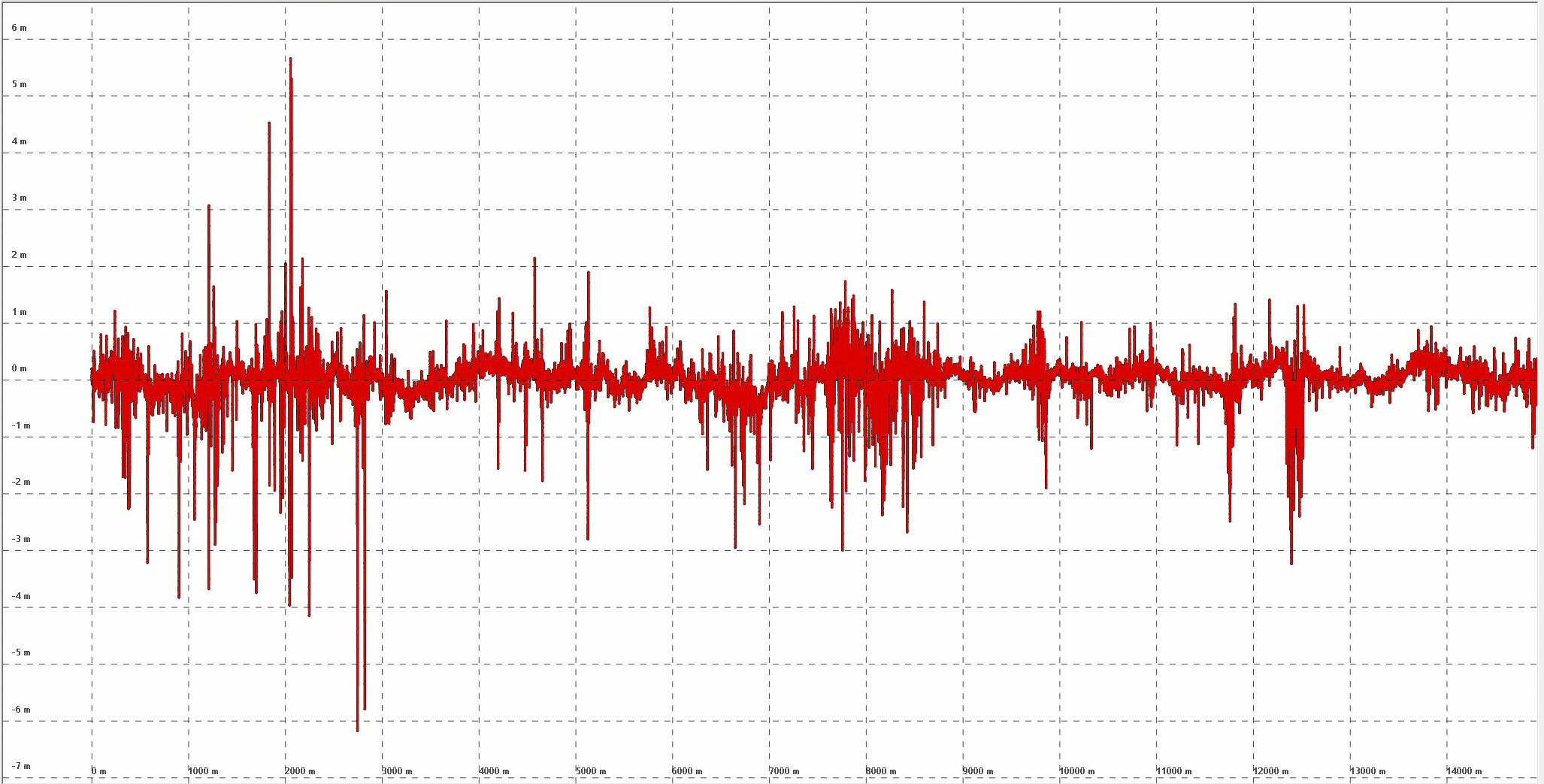
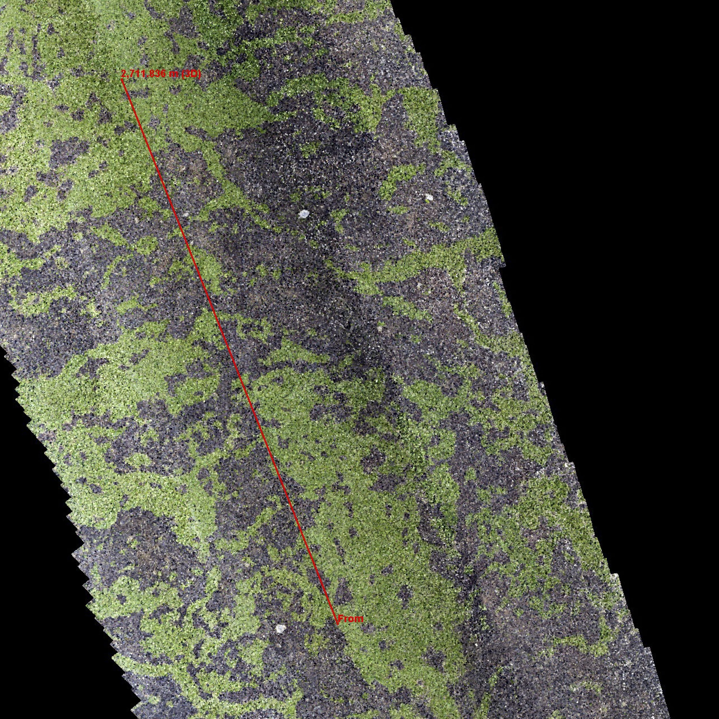
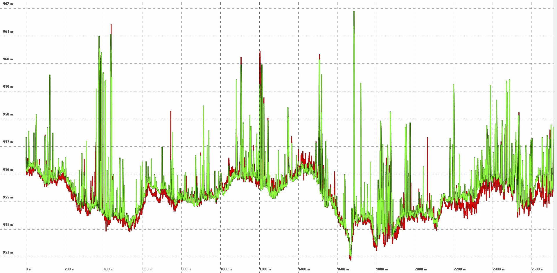
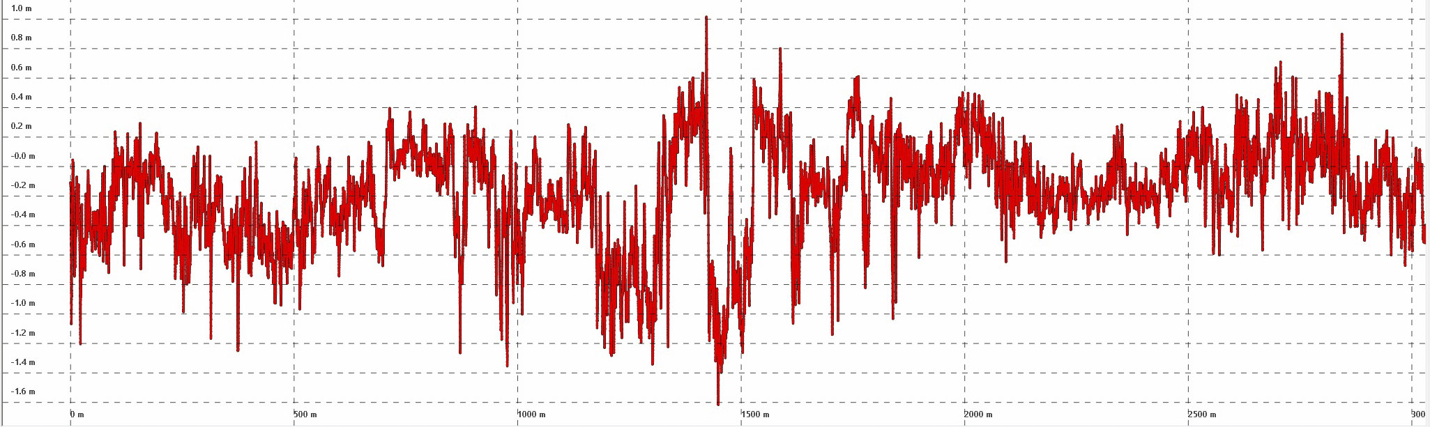
Here are the elevation differences along a 15 km long transect. The large differences here are caused by the difference in leaves — in 2018 most of the trees had not leafed out yet, so at this resolution the fodar maps are looking at the ground instead of the canopy. The mean misfit here is about 50 cm with 95% of points being about +/- 50 cm. So at least we know the geolocational accuracy is within 50 cm, but we need to look at smaller transects to eliminate the confounding factors of vegetation.Here I have overlain the point clouds from both the high and low transects together and run a transect through, with elevation value shown below.The horizontal grid lines here are 1 m apart, so you can see that the differences in ground elevation in the 2.6 km long transect are in the 10-20 cm range here. Given that these transects were made from independent data and given the wealth of prior analyses, I think we have good reason to believe that geolocational accuracy here is better than 30 cm as usual; a few ground control points would reduce to that to the precision level of 10-20 cm.
Here I discuss two methods of ground control involving ground photos using the same example. As I progressed with ground-vehicle technique development, I experimented with creating fodar point clouds from the ground to compare to the airborne one, for utility in geolocation accuracy determination, canopy structure measurement, and canopy shape technique comparisons. These same photos, as well as the ones not acquired in this way, are also useful in determining species type from the airborne data, as the ground photos resolve tree and leaf shape better.
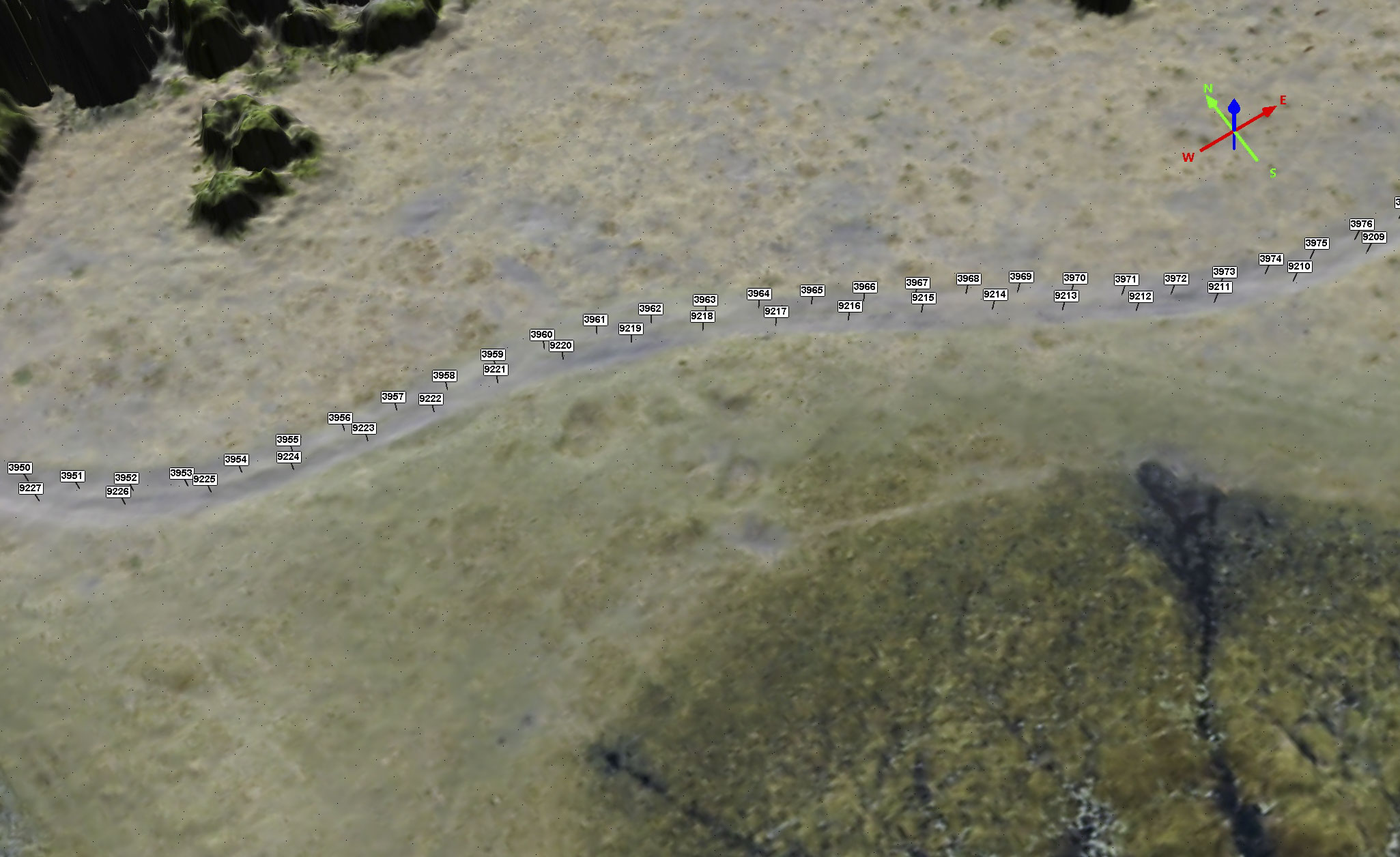
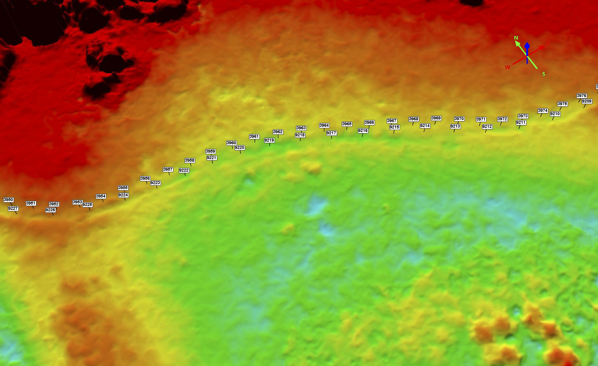
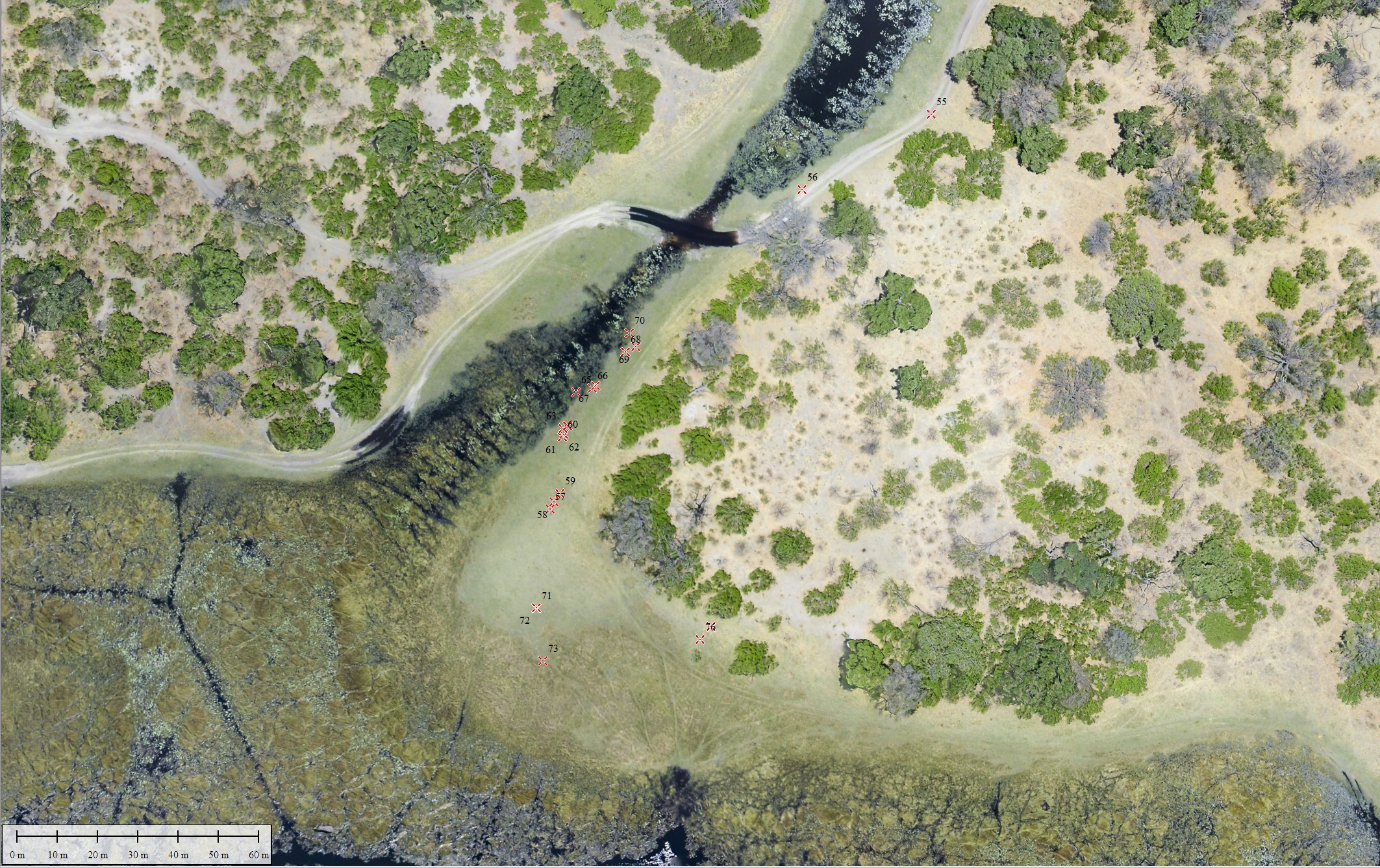
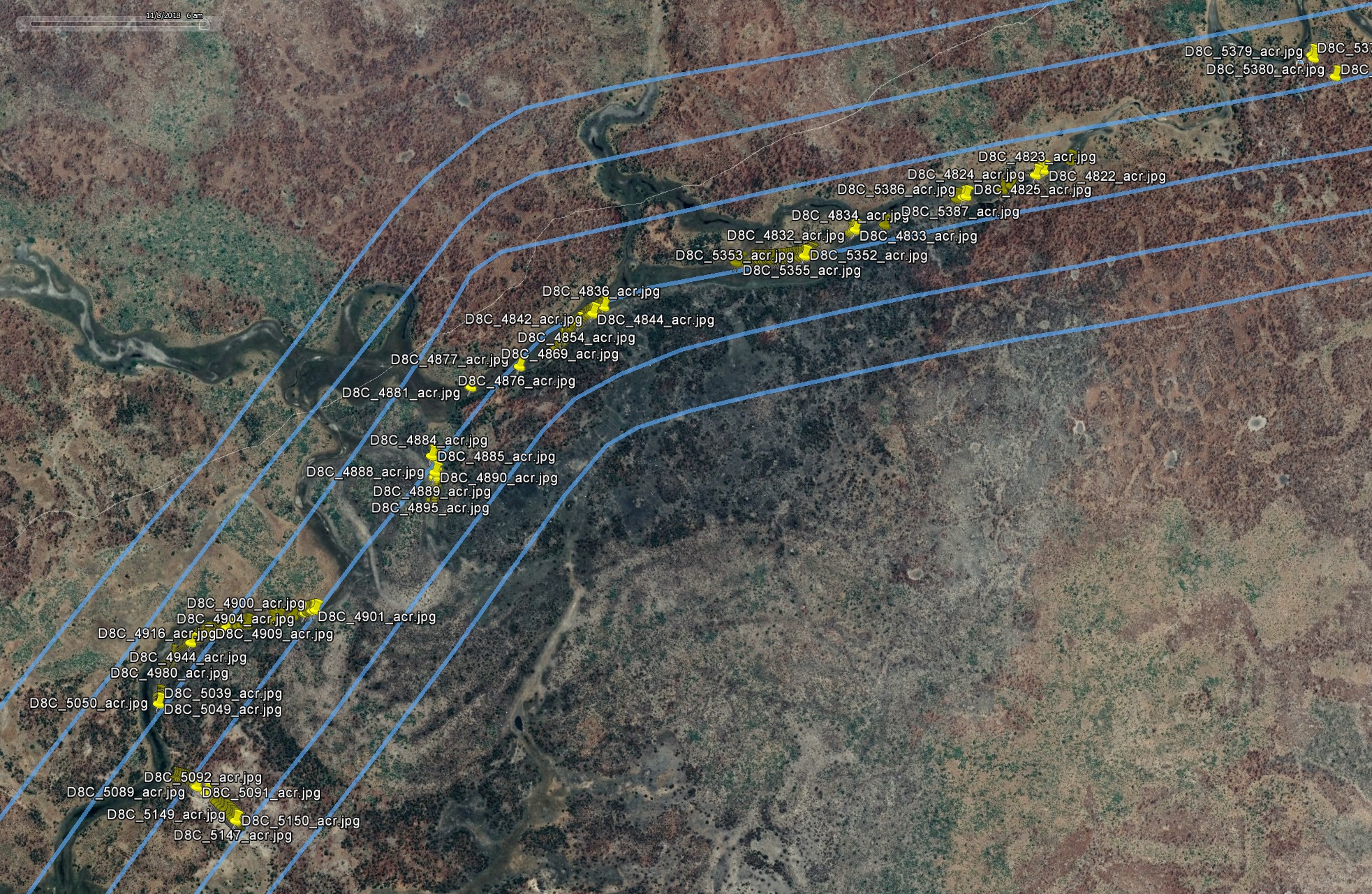
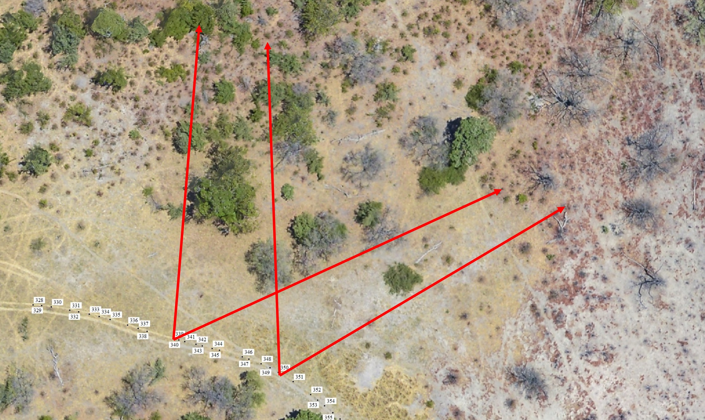
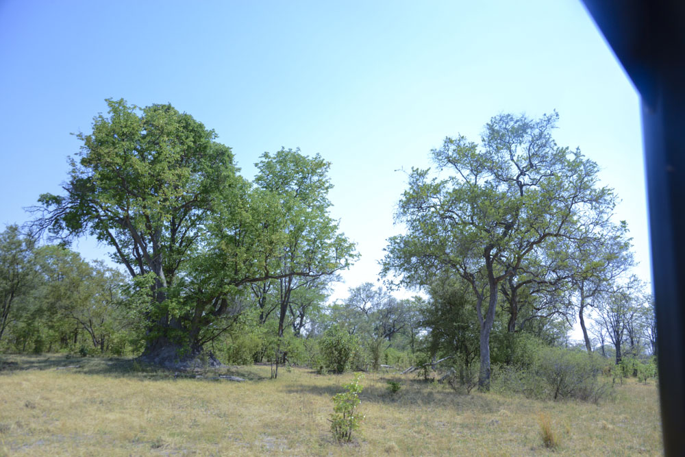
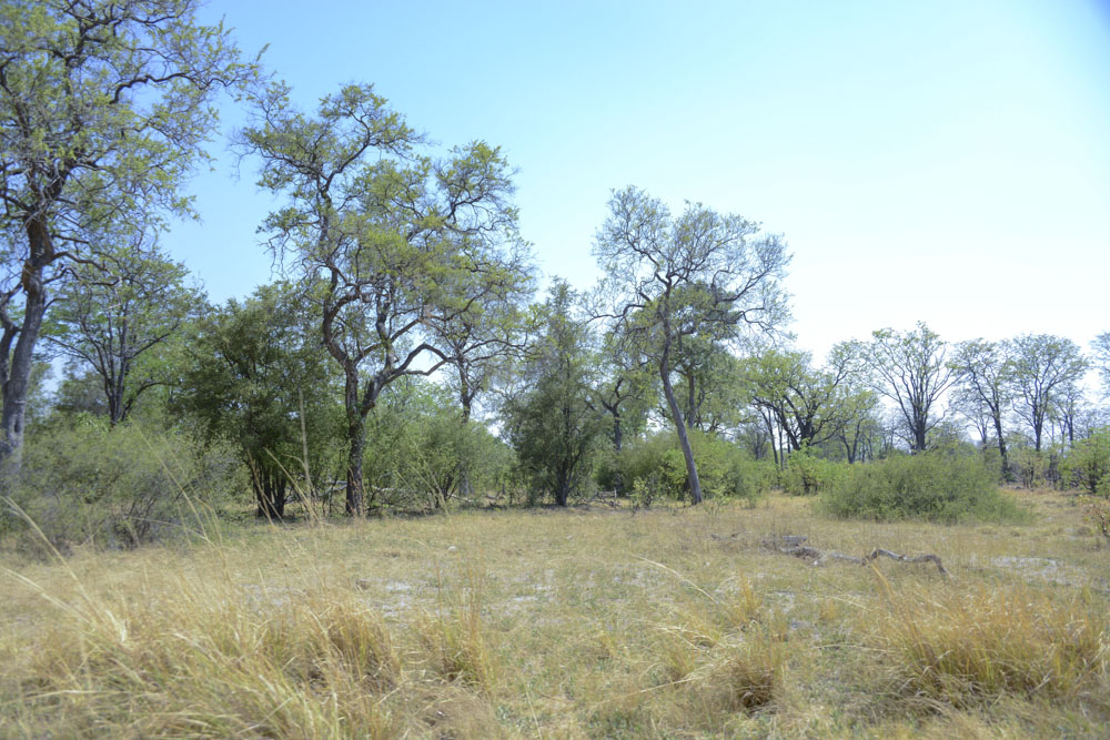
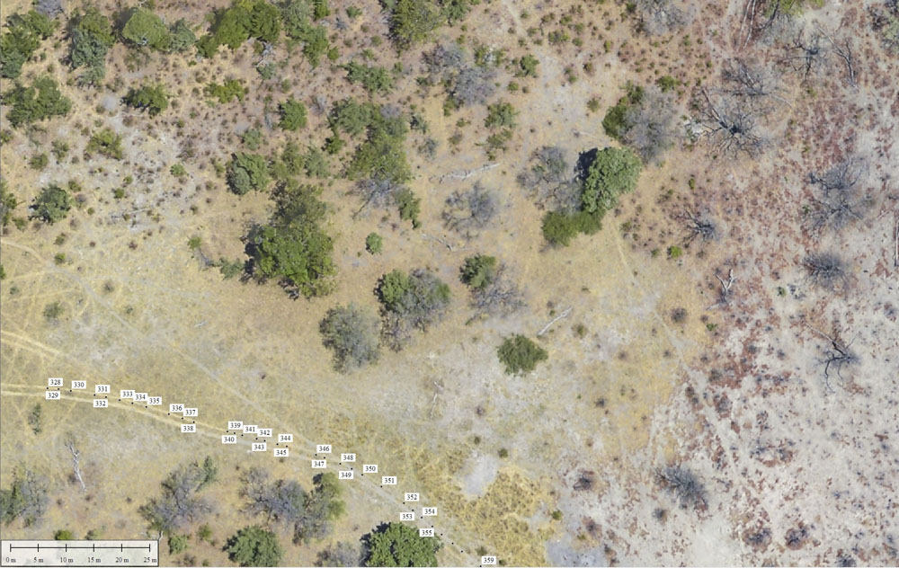
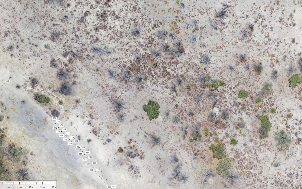
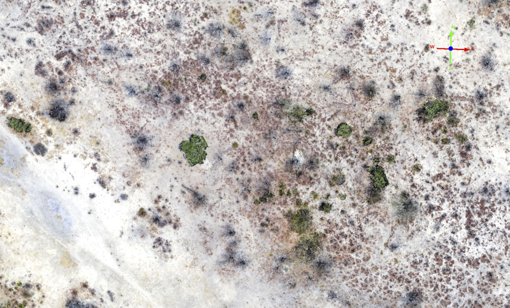
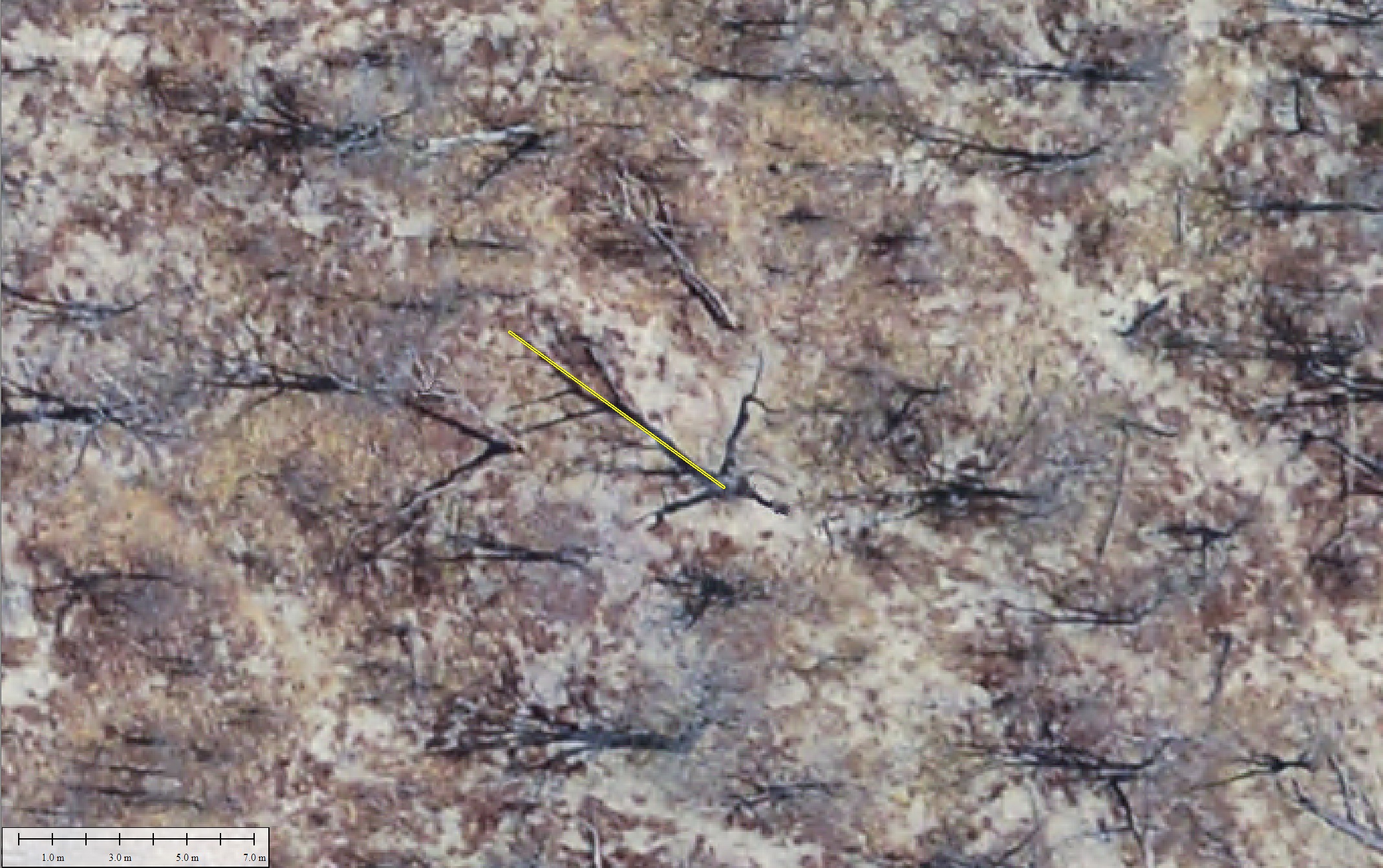
I attached the camera to the rail of the safari vehicle using some very adaptable clamps I brought to test new ideas like this as they came up. Here the camera is attached to a high resolution GPS to give me the same precise position as I get in the helicopter.Here is an example of photo locations (yellow pushpins) on one of our drives, relative to our flight lines (blue), as seen in Google Earth. You can click on these pushpins to see the images.Here are a selection of photo locations (numbers in white blocks) over the fodar orthoimage, near the Selinda spillway. The red arrows indicate the approximate view of the next two photos. The idea is that these photos can help with validation of species identification using the orthoimage.Here is photo 340 from above.Here is photo 350. This photo overlaps slightly with 340.Here is that same snippet of orthoimage again, for comparison to the point clouds below, against which I can make vertical measurements. The orthoimage has more clarity and definition I think for a variety of purposes. These photos are what I used to make the ground-based point clouds in the next few analyses.
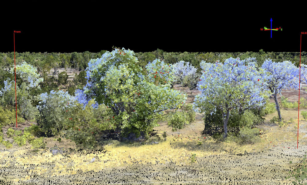
At left I have overlain the ground-based point cloud over the airborne-based point cloud. The ground one has a lot of blue in the leaves, as I was looking up into the sky through the leaves (see photos 340 and 350 above); I can filter that blue out, but I left some of it in as I thought it improved clarity in distinguish the two point clouds. This view captures the same area as shown in those two photos. One thing to note is that these ground photos were acquired 10 days after the airborne data, and many trees turned from leafless to leafy during that time.
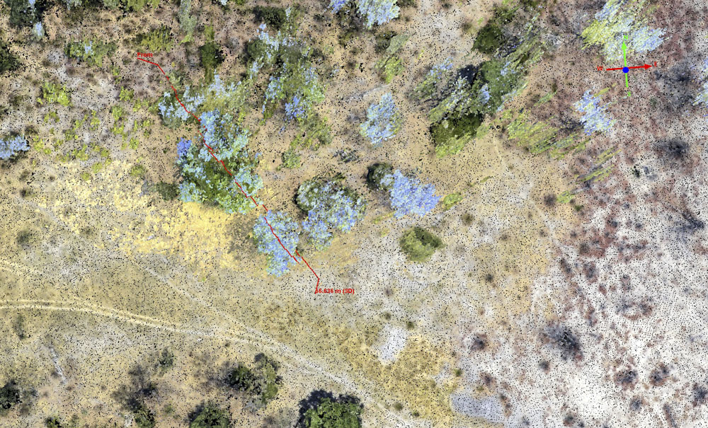
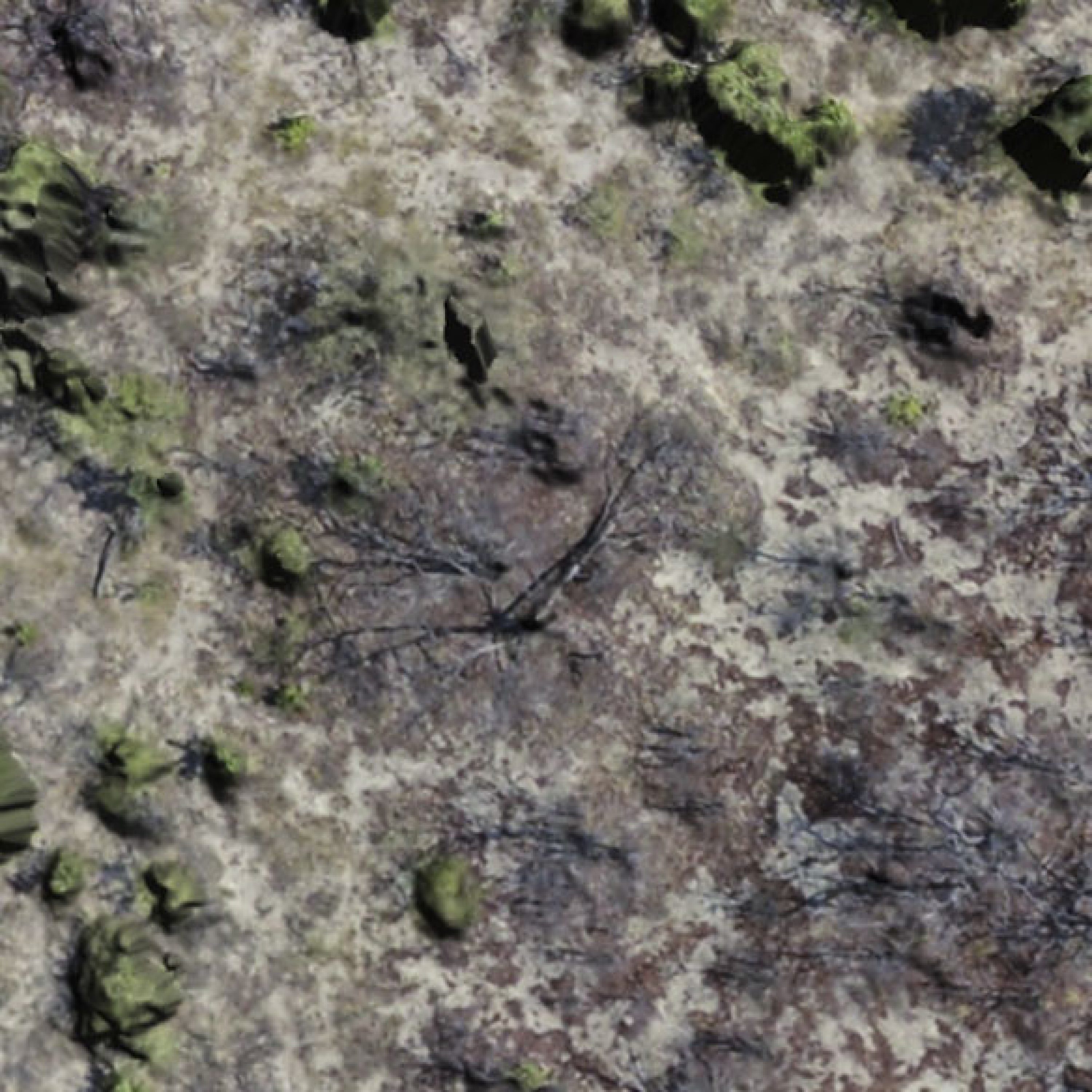
Here is a top view of those two point clouds. I have drawn a transect over the top of the tallest tree, which you can see in the left side of photo 340.Here are the elevations extracted from the transect above, the red points are airborne and the green ground-based. At left, you can see that the back of the tree was blocked from view from the ground, so there were no points there. The large tree in center is captured similarly in both cases, noting that from the air the lower branches are obscured from view and from the ground the far side of the tree is obscured from view. The ground data can be improved by circling the trees. The two techniques might be complementary in that they could processed together, not something I have rigorously tested yet. The tree at right was largely leafless during airborne acquisitions (see orthoimage) as you can see the airborne trunk poking through in red but had fresh leaves had sprouted once we reached it by ground (see right side of photo 340). There was a slight misfit vertically between the two techniques, which I corrected for manually as there were several shortcuts I took in getting this far for this blog.Here is another stretch of orthoimage and photos, maybe 300 meters south of the previous examples, which I made the point clouds below from. Notice that the bulk of the trees in the orthoimage are leafless, and from the red leaf litter you can tell they are mopane.Here’s a photo from that strip. It may be hard to tell, but the leaves are just starting to pop out on the stunted mopane trees.
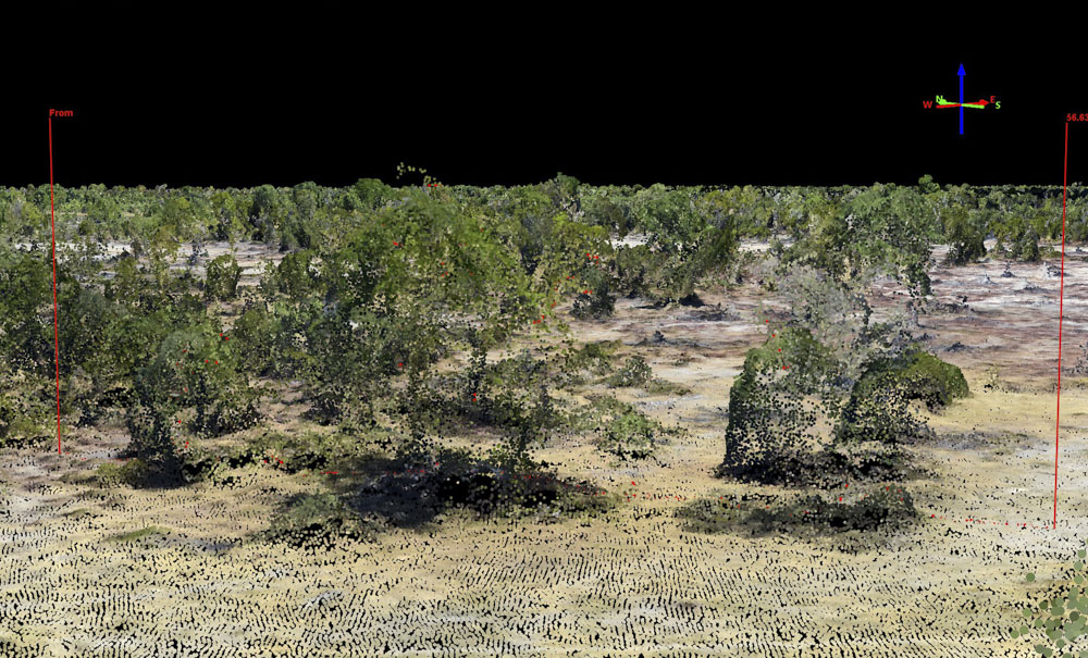
Here is a top down view of both point clouds, roughly matching the perspective in the previous orthoimage. Notice how many more blue (ground-based) trees appear. This is in large part due to the emergence of leaves, but also the increase in resolution, in this case 3-5 cm compared to 20 cm.
Here is a perspective view of the same data in the previous comparison. Here you can clearly see the differences leaves and resolution make, as not all of the trees have leaves yet. The point is that time of year matters and that resolution matters — the differences here have nothing to do with the quality or capabilities of the technique. Indeed, the fact that the same equipment is revealing these differences indicates that the equipment and technique are not responsible for them, it’s really just knowing how to use them to optimize results and cost. In this case, the thin diameters of stunted mopane trunks and branches are below what can be resolved at 10 cm image GSD from the air, but flying lower or driving next to them is sufficient to resolve them. Doubling the resolution (5 cm instead of 10 cm) roughly doubles the flight time and costs, but for these transects that’s only $1500 so it’s always important to keep actual costs in mind rather just percentage increases. The question then becomes does the extra $1500 in cost increase the value of the science by including leafless mopane in the elevation results? I address this further later.
I believe these tests paint a picture consistent with all of our previous studies — these data have a repeatabililty of better than +/- 20 cm at 95% and a geolocational accuracy of better than 30 cm, which can be reduced to the level of precision with quality ground control. My ground data was overwhelmingly sufficient to validate the horizontal accuracy and precision and vertical precision, but only mediocre in vertical accuracy due to some issues I had with my hokey ground system. An equally important point is that I got a great start in developing cheap methods for ground control, such that on my next trip I can implement something more efficient and reliable. These tests, as well as some below, also indicate that resolution (more properly Ground Sample Distance or GSD) and timing relative to leaf out are controlling factors in resolving the shape and structure of woody vegetation.
Sample Analyses
The main point of this blog is just to say that everything worked great on the technical side, but of course it is difficult to resist doing some sample tests to see how these data can contribute to our overarching questions about elephant habitats and dynamics, including exploring options we might consider for the future. So here are just a few quick examples I did while processing and validating the data, along with a few thoughts of what we could do next, in addition to what I have discussed already.
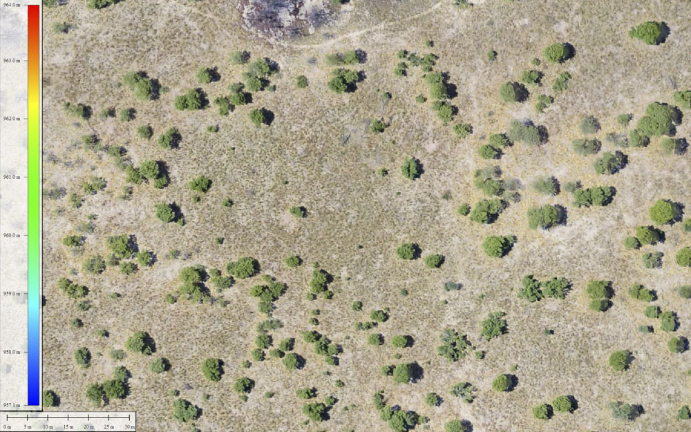
The goal of the project was to measure tree height as function of distance from water bodies and how it varies over time. I’ve already given a bunch of examples of measuring tree height, such as in the videos, but here is another just demonstrating that everywhere there is leafy vegetation (left, orthoimage) we are also measuring its topography (right, digital elevation model).
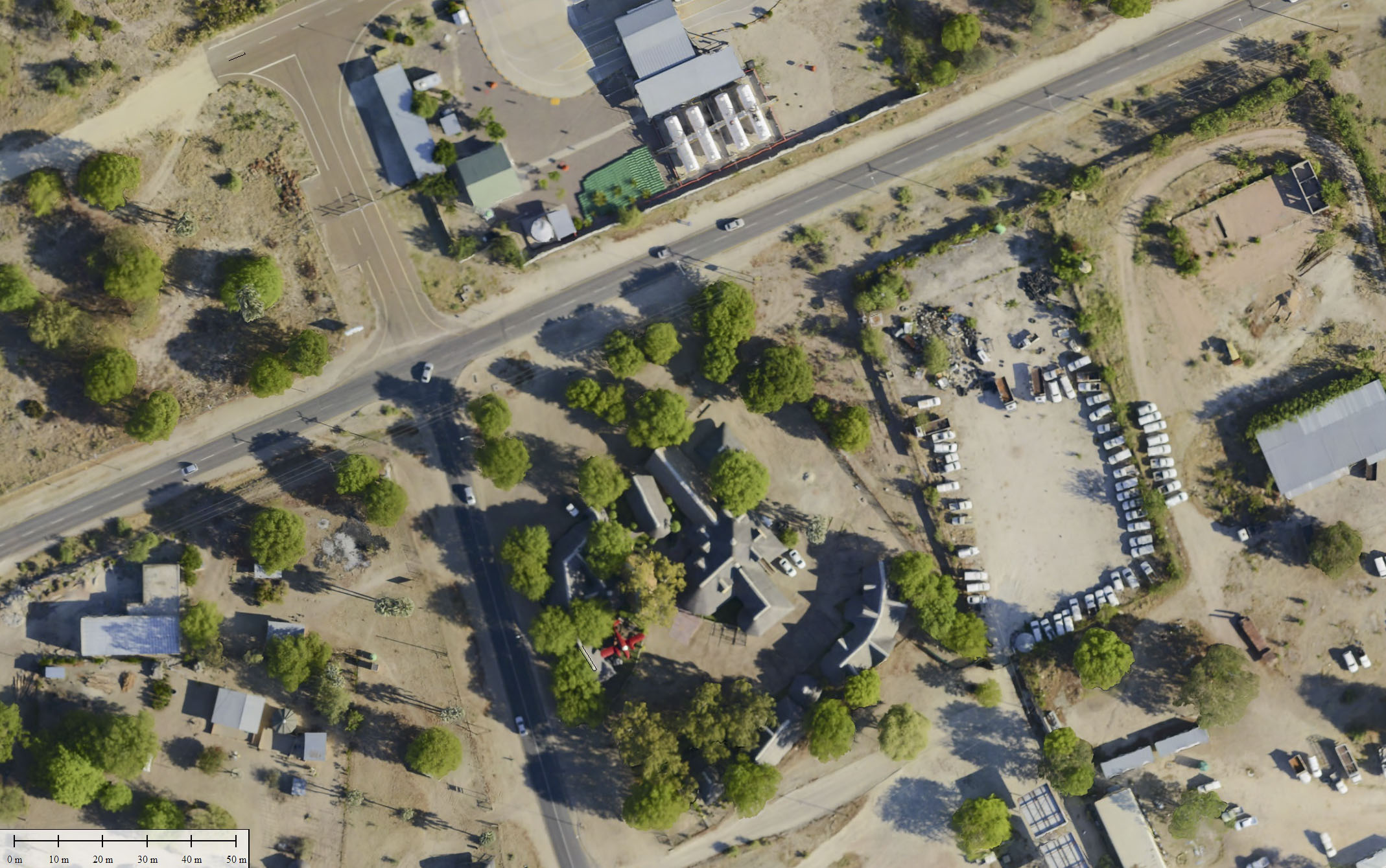
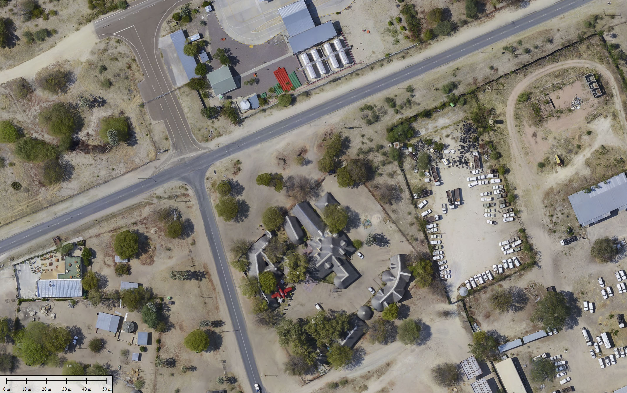
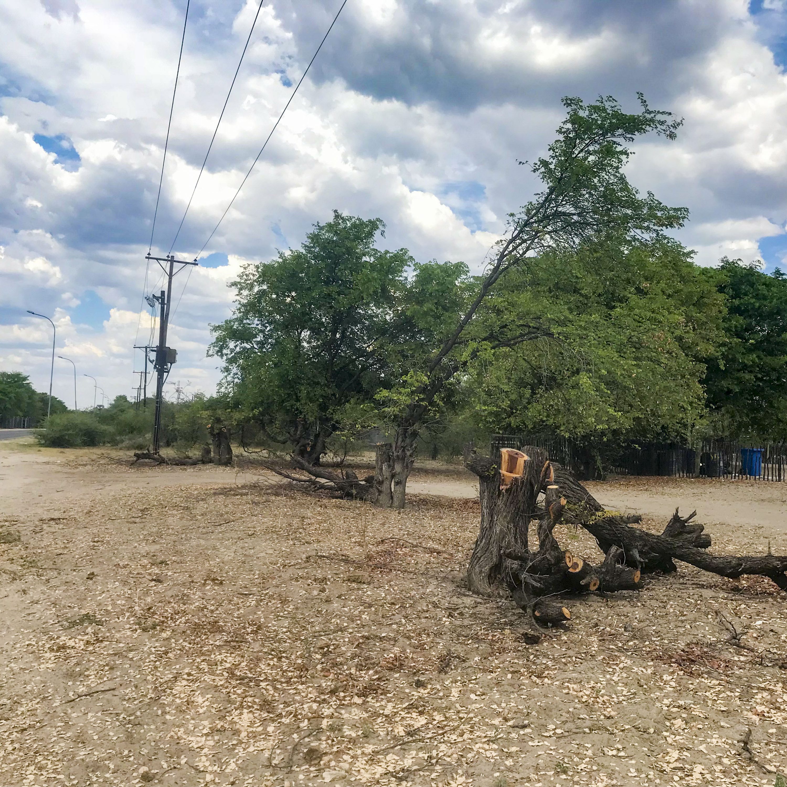
Sometime between our November 2017 and November 2018 visits, several mopane trees got knocked down in front of the Tandurei restaurant, one of our favorite hangouts, to limit interference with power lines. Thus it makes a convenient local site for testing tree dynamics in the wild, since I know what happened on the ground and could access it. So I’m using what happened there as an example of what elephants do in the field.
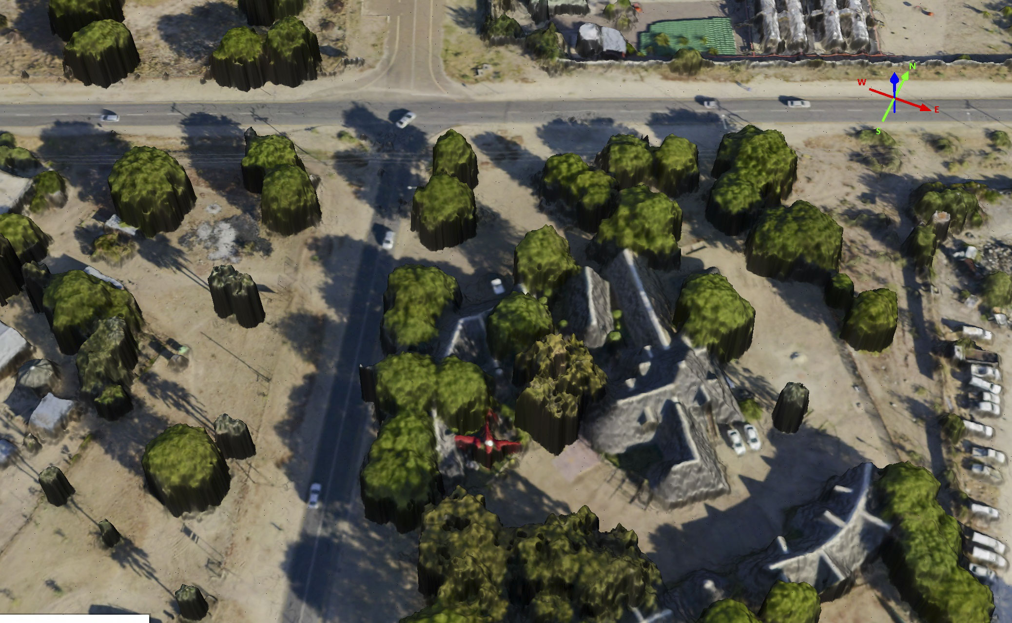
The Tandurei is the complex of buildings just below center with the red airplane in the parking lot. Just north (up) from there you will notice several trees have been removed, as well as kitty-kornered across the street to the left. So right away we know that the fodar imagery alone is capable of seeing when trees disappear.
Here are those exact trees in front of Tandurei. Notice one removed completely and another only about half; you can see this in the data clearly.
Here is an oblique view of 3D fodar data — here the image data are overlaid onto the topography. Note how we can easily we can see the change in shape of trees (if you look closely you can see most appear to be thinner, due to less leaf canopy growth in 2018) or their elimination completely with these data (see upper left and just up from the Tandurei courtyard)
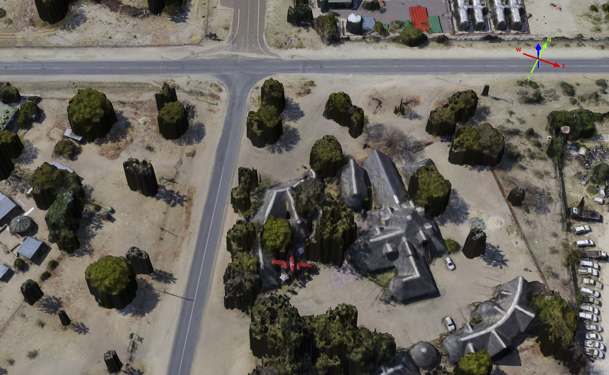
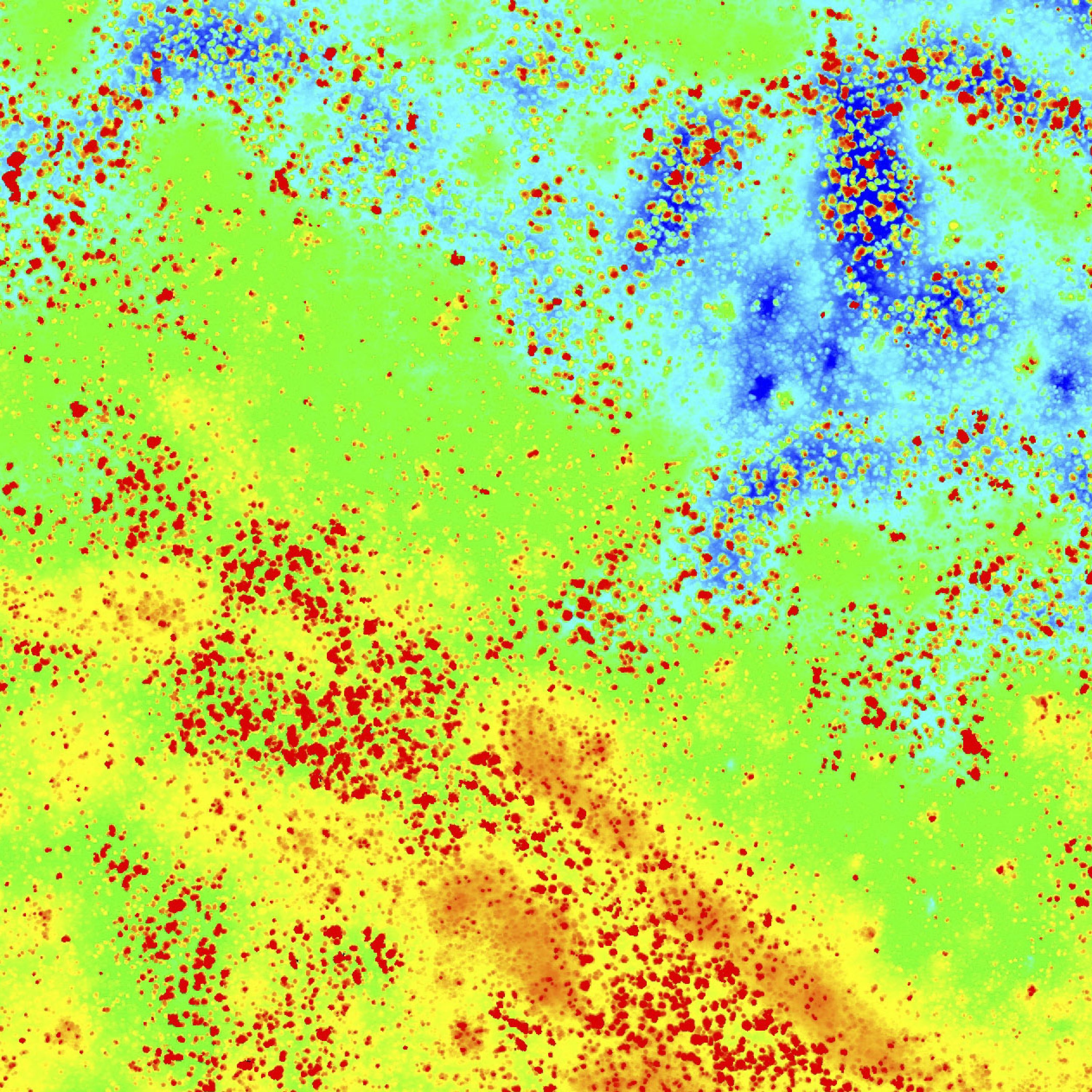
Here are those same data, this time without the image overlay. Blue is low elevation, red is high elevation. Note that Digital Elevation Models (DEMs) like these using any data (fodar, lidar, insar, etc) are incapable of resolving two elevations at once (like underneath a bridge or tree) so the tree canopies here come straight to the ground.
Here is the difference between 2018 and 2017 topography, with red meaning little to no change and blue meaning something disappeared in that interval. The trees that were removed now show up very clearly as pits (greens-blues). However, in 2018 the leaves had only just begun popping out, so the canopies were not as full. This difference in tree shape is manifest here as a moat of greens-blues around many of the trees. In this case, these moats are a form of noise if all we are looking for a trees that have been knocked over by elephants (or construction workers). But the beauty of this sample study is that it demonstrates that we can also measure a change in tree shape caused by elephants if we make our repeat measurements when leaf maturity is in a similar state. For example, just pretend for a moment that leaves popped out on the same date each year and matured at the same rate, such as if our 2017 and 2018 data were made on the same calendar day, this analysis would indicate that a herd of elephants or giraffes or tree trimmers came through Maun and took a few feet off the diameter of each of these trees. That is, this sample analysis indicates that there is almost nothing happening with tree shape that we cannot measure through repeat measurements. In either case, it would be relatively straightforward to write a script that would analyze difference images like these to search for pits and moats to identify and quantify the impacts of elephant browse on the landscape.
Trees are not the only vegetation we can measure change in. Here are the Boro River maps we made in 2017 and 2018. We took a mokoro trip here in 2017, and still remember some of the individual features and trees that we saw then. Here you can clearly see some differences in vegetation related to differences in the timing of flood dynamics, which are localized around the river.
Here is a stretch of the waterlogged part of the acquisition. The colors at right are +/- 50 cm of elevation difference between the 2017 and 2018 data. You can see how the color distribution is not random or aligned with sharp photo edges or corners — these are real variations, largely caused by marsh grasses I believe.
Here you can see the changes in height over the red transect in the previous image pair. These values are well above the noise level we previously demonstrated, so are likely real. But they are not so high as to be differences in trees, but rather I think grasses an shrubs.
This is from a different location, but gives the general sense of what these swamp grasses look like.
Here is a drier section of our acquisition. On our 2017 mokoro trip, we hiked into this area, and used our ground photos to compare with the airborne data.Notice in these elevation differences, the values are much smaller and closer to the noise level. I believe this is due to the dry-land grasses not having a seasonal height variation as strong as marsh grasses. It is difficult to say whether the difference in mean values is due to a true environmental difference or a system bias, but to the right of the vertical red line you can see a consistent rise in those values; this corresponds to the start of the burned area (southern part of transect), and likely represents the new growth in grasses there in 2018. Thus fodar could make measurements that support the habitats of grazers, like wildebeest and zebra.Here is an example of the marshy grasses that grow alongside the Boro River, which apparently have seasonally-dependent growth.Not only can we measure changes in grass height, but also changes in water height. There is enough flat, floating vegetation like lily pads in the water that we can measure their elevation photogrammetrically as a proxy for water height, as I show later.
One of the primary objectives of this study was to determine the height of trees as a function of distance from the various swamps. In the previous examples and in our 2017 study, we demonstrate that this no problem for trees with canopies. As fate would have it, during our 2018 visit most of the mopane were bare and the terminalia had just started sprouting. In 2017, I didn’t know anything about Botswana ecology and was here only to demonstrate cool things fodar could do, so I didn’t realize at that time that the bare mopane trees were even alive, so I was mostly thinking about mapping tree canopies. In 2018, the focus of my learning experience here was trees, but it was not until we were actually airborne that I learned that these leafless mopane were actually alive and a primary food source for elephants. Given what I saw on the ground about their size, I suspect we planned our flight lines too high, optimizing for spatial coverage over resolution. So on our last flight, I added a few lines at lower altitude so we could assess best methods for the future. In this case, I changed ground sampling distance of the imagery from 10 cm to 6 cm, and show some results below.
Here are views of point clouds of different resolution from NG18B. Though the difference is only 4 cm in GSD, because the leafless branches of these mopane are so thin, the lower resolution makes a big difference in capturing them digitally. If we wished, we could also digitally filter out all of the trees so that we could studying hydrology, such as the tree filtering I demonstrate in this blog.
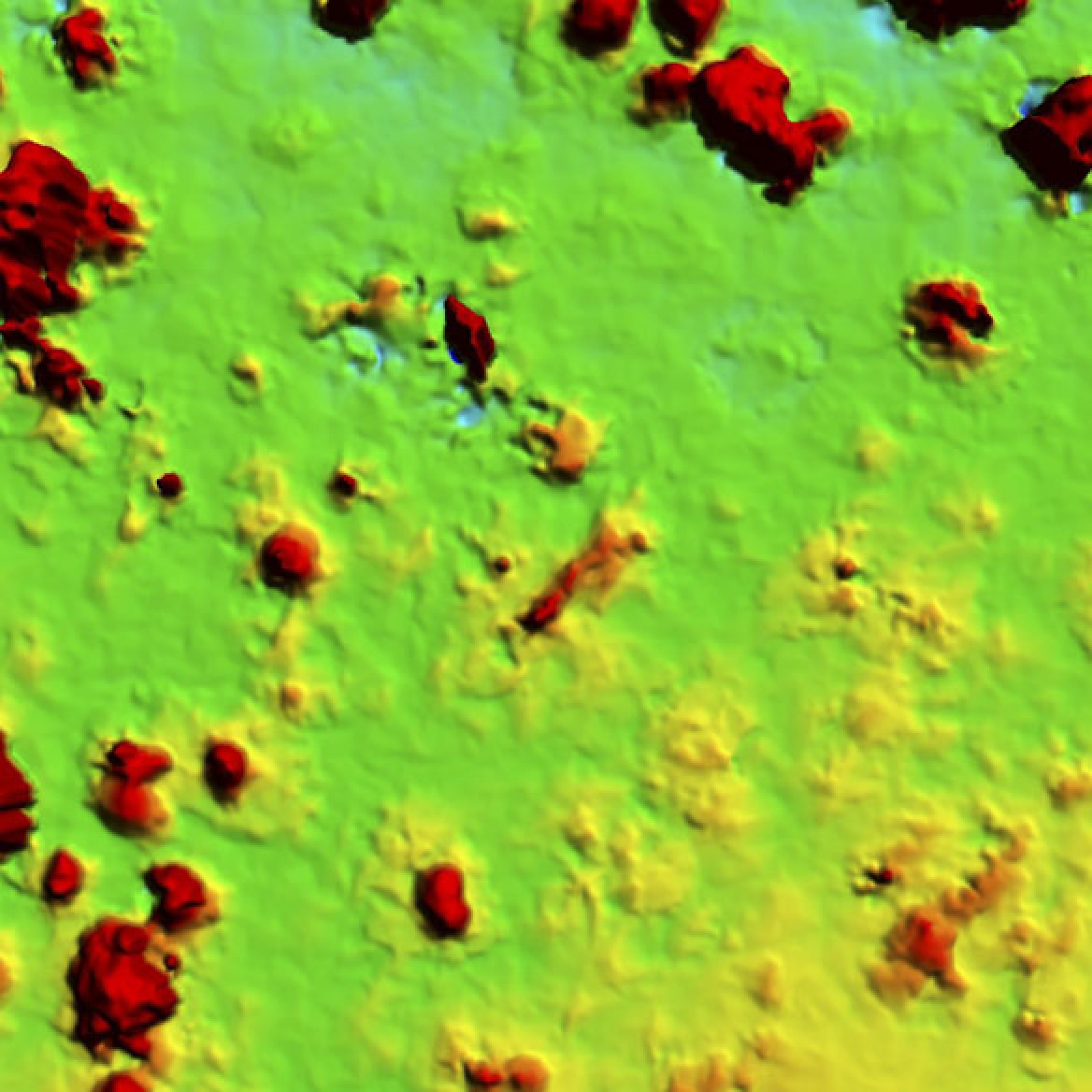
Here is another way to understand the improvement that higher resolution makes. These are the two point clouds made from different flying heights, with red colored as high elevations and mostly indicating the location and height of trees. As you flicker between them, you will notice that there are more red dots (trees) visible in the higher resolution data, and also that larger red dots at 10 cm turn into several smaller red dots at 6 cm as clumps of trees get resolved as individual trees. You will also see a color change in many dots, as higher resolution data will resolve the height of a small spiky tree better than lower resolution, meaning that measured tree height will be a function of resolution for leafless trees. Note that this is not revealing a deficiency in fodar, as such spatial biasing issues are common to every technique, but rather simply why and how resolution matters so that the best optimizations between time, money, spatial extent, and analysis abilities can be made.
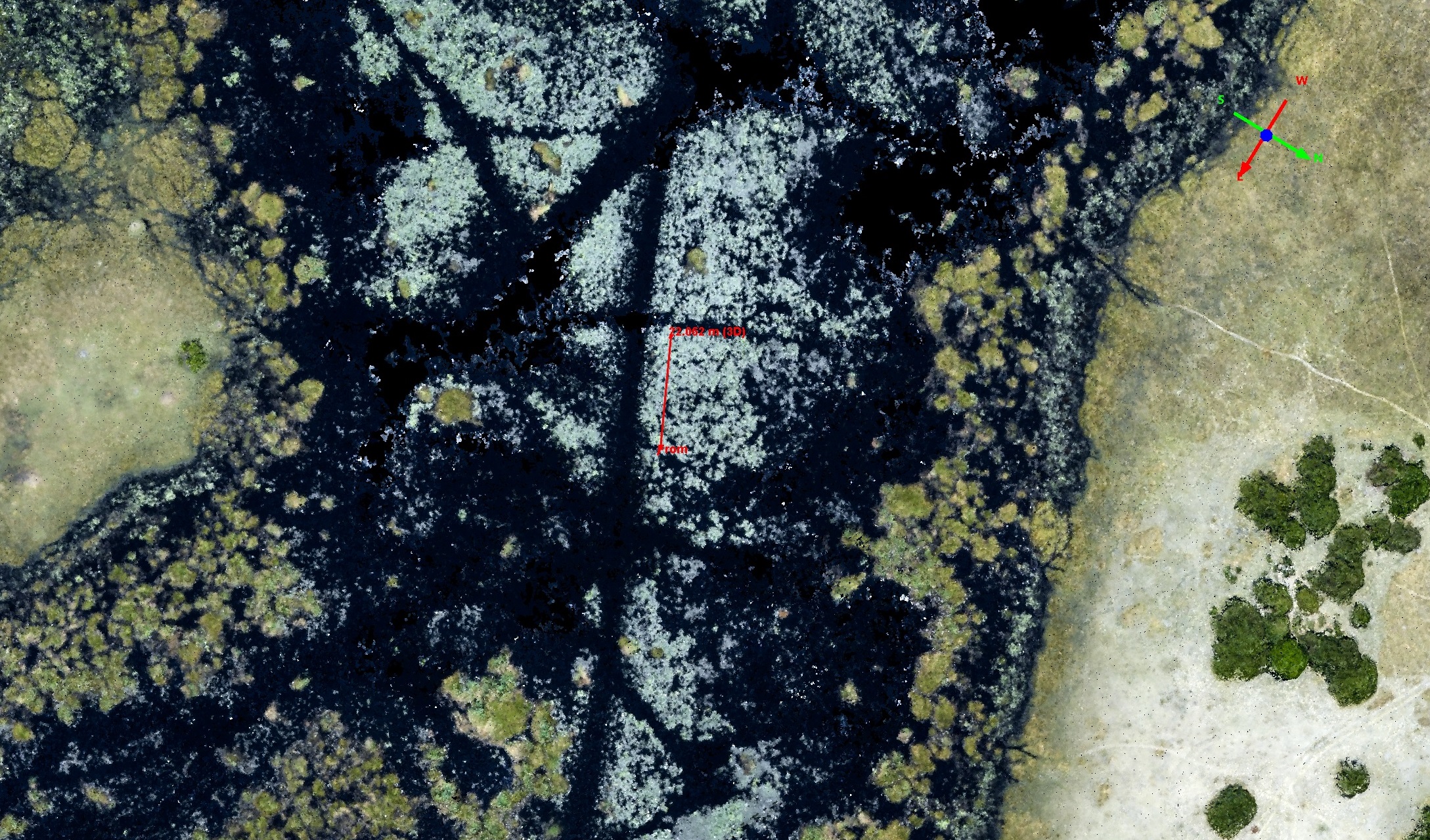
Even when a tree is too thin to be resolved in topography at a given GSD, it is still possible to measure it’s height using it’s shadow. Here I have measured the distance from the base of a tree (near center) to the top of its highest branch as about 8 m. On November 8th at 10 AM at this location, the solar angle predicts that to create an 8 m shadow the tree would have to be 2.9 m tall. Fortunately it was sunny during most of our acquisitions, so though it will take some manual effort compared to acquiring the data at a higher resolution in the first place, it should still be possible to measure the height of nearly any tree here regardless of whether the trees are resolved in topography. Note that this only works because the fodar images are orthorectified into a mosaic, such that the mosaic has a uniform scale throughout. That is, don’t try this with just any photo, as the warps in perspective will skew the result!
Here is an example of determining when a tree has been knocked down (near center), using its shadow (left) and its elevation (right).
Though fodar cannot measure water surface elevations accurately, it can measure the elevations of things floating in the water accurately and their elevations can be used as a proxy for water surface elevation. In the example below, I show how lily pads are a great proxy along these lines.
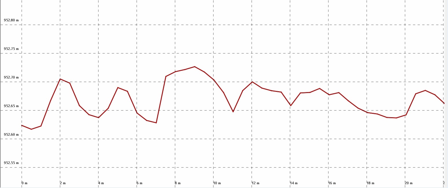
Here I’ve zoomed in on some floating vegetation that is nearly flat, like lily pads, and drawn an elevation transect over it.Here is the elevation transect from the previous image. The elevations here are 957.67 m HAE +/- 5 cm, and that’s as good as I can pick from studying the shorelines here. This vegetation is only a few centimeters above the water level, if that, so this method should be as accurate as any other in determining water surface elevations distributed over large areas. For example, further down the Selinda spillway from here where the last connected open water was to be found downstream of this location, I measured only about a 40 cm drop just before it dried out. Given we measured dry channel after that, it would take a pretty simple computer model to determine the future extent of connected open water as a function of stage. Also, given that we can measure lily pads, swamp grass heights with no problem, and given how these can detach and block channels and create new landscapes, this may open up new areas of investigation.
The Future
My analysis of the 2018 fodar data shown here is that it technically performed exactly as planned and that this opens the door to a wide variety of future work. We discovered here that the measurement of tree heights is possible from the elevation data when the proper resolution is selected and complicated by temporal variations in leafiness, but with proper care in planning these constraints can be overcome as the change is logistical not technical. In this and our 2017 work, we learned that we also measure the subtle variations in topography that control hydrology here at the process level, such that we also measure topographic change at the scale that allows us to predict changes at the process level, whether that’s making flood inundation maps using the dry topography, measuring dry pans as bathymetry to determine their volume later using only a photograph, or measuring water levels in the swamps in realtime using the floating vegetative mat as a proxy for water height then determining flood water volumes by comparing it to the dry topography as bathymetric hypsometry. Previously we also determined that we could not only identify and count large mammals in our data, but measure body morphometrics using the topography.
In 2017 we spent some time mapping animals to see how well it would work. So this video is not an actual video or something from a drone, this is a 3D visualization of our fodar data.
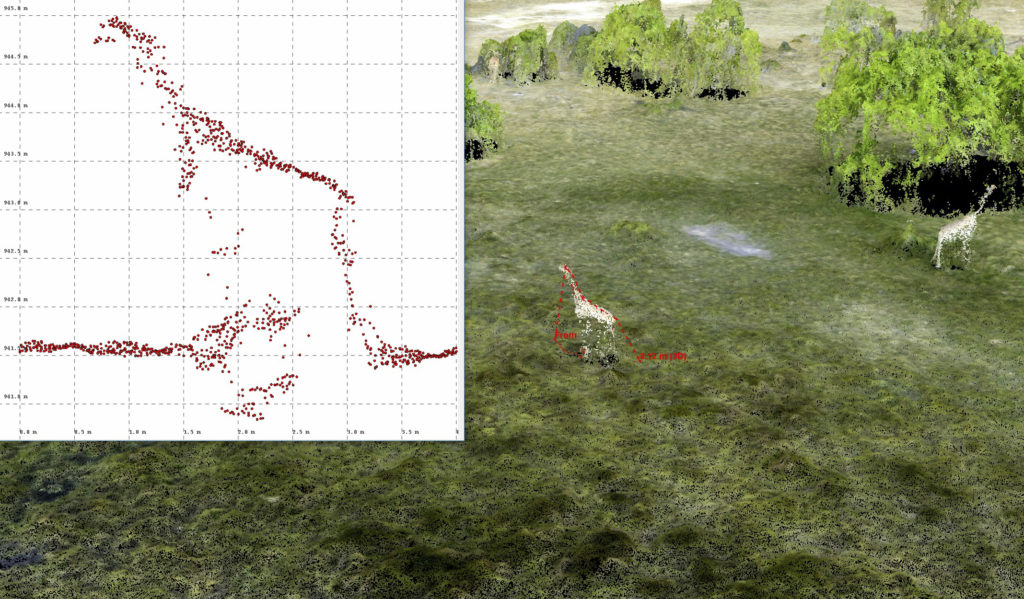
Using fodar, game counts could become much more than just counts, we could measure size too. Here’s an example of measuring giraffe height using fodar data, from 2017. We could potentially be doing this across the whole country. The trick in 2017 was that the animals had to be standing still between our back and forth passes; using 10 helicopters flying side by side eliminates this constraint.
Here is a similar example using elephants. By mapping both the game and the landscape at this resolution monthly over huge areas, we can begin to answer much more sophisticated questions about wildlife ecology, as described below.
All of these findings to me lead up to an intriguing and potentially game-changing possibility — we could map the entire Okavango Delta in 2 days using the entire fleet of Helicopter Horizon’s ships to limit temporal change during the acquisition, then do this on a monthly basis to capture the full range of seasonal variation in ecological dynamics between landscape, hydrology, botany, and wildlife. The price to equip 10 helicopters with my fodar systems and operate them like this is far less than a single lidar unit costs to purchase. That is, flying 10 helicopters in echelon formation reduces our mission duration by a factor of 10 without increasing our flight time, allowing us to capture swaths 10x wider, effectively eliminating double-counting of moving game while simultaneously eliminating under-counting since the counting is occurring in the office rather than visually while in the air, with the bonus that we can not only count elephants and nearly all game visible at the selected resolution but also get information on their size and health, and does so operationally for less cost than simply buying one unit of the state-of-the-art alternative with no sacrifice in quality. Doing this monthly for a year allows us to asses the changes in distribution in game as they may relate to changes in flood stage, vegetative state, etc. For example, we can not only learn the seasonal impacts of elephants on woody vegetation, but we can determine how long their presence in a particular area relates to their impacts as a function of vegetation type or even individual trees. As another example, if we compare such game counts to traditional game counting methods, we have a means to assess that method and apply those finding to past or future counts using that method. But of course, these are ideas on African ecology coming from an Alaskan glaciologist, so how valuable such analyses are is beyond my expertise to say, I’m just opening the door to discussions on that by saying that these analysis are technically feasible should they be deemed valuable.
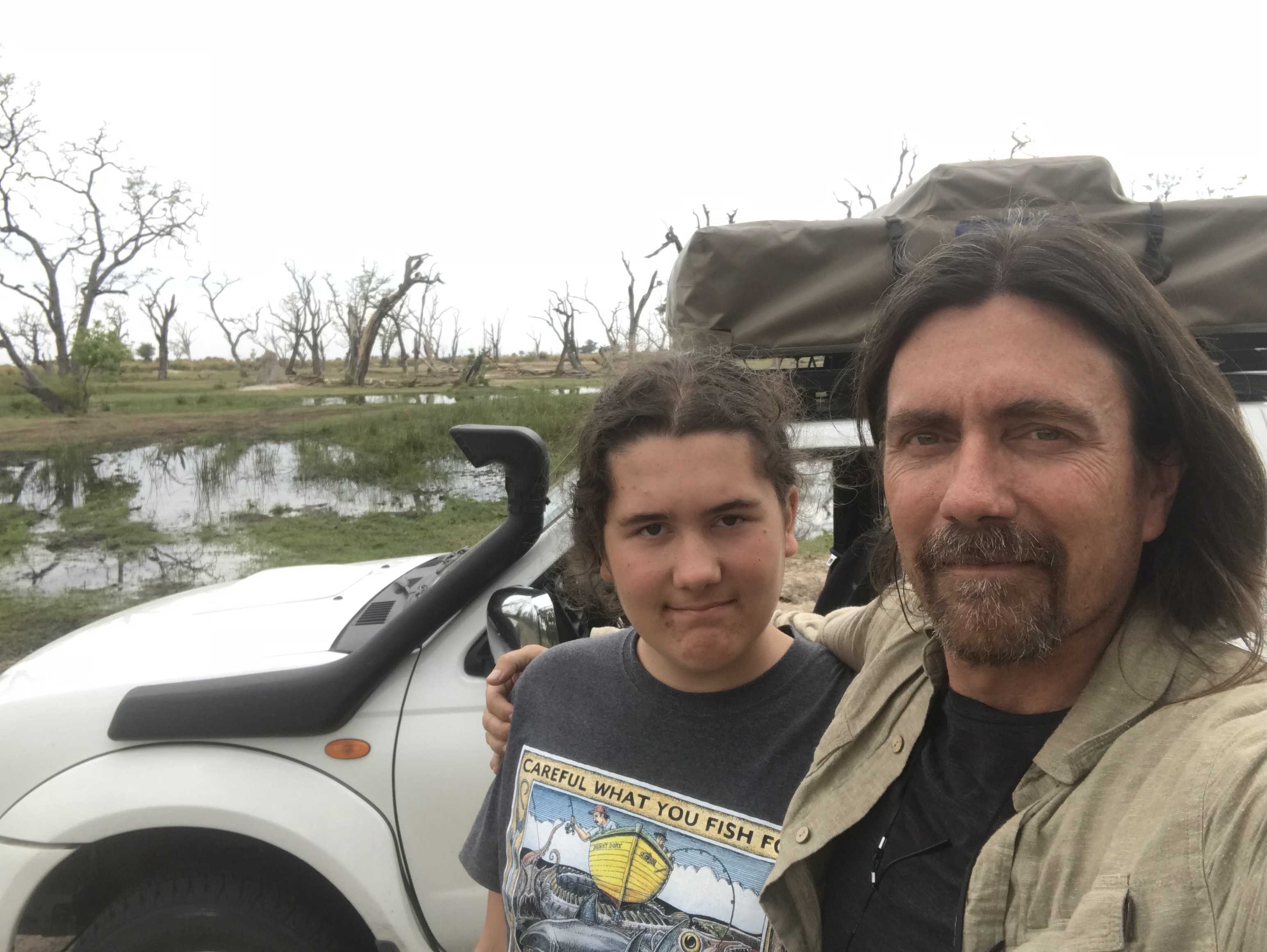
If there was enough interest, we could map the whole country like this in a week. But as Turner reminds us,”Careful what you fish for”…
Contact Us
We're not around right now. But you can send us an email and we'll get back to you, asap.


