
What is Fodar?
This page presents a review of the important concepts and terms related to fodar and digital photogrammetry. Note that fodar is not an acronym and is not capitalized, it is simply a term I coined as a convenient portmanteau of ‘foto’ and ‘lidar’, just as ‘lidar’ itself is not an acronym but a portmanteau of ‘light’ and ‘radar’. I define fodar as any photogrammetric process for quantitatively measuring both the color and elevation of the earth’s surface from the air using a small-format digital camera.
As we implement it, fodar is an airborne photogrammetric technique for making high resolution topographic maps with sufficient accuracy and precision that by subtracting two of these maps we can detect changes to the ground surface on the order of centimeters. It works by flying over an area of interest, taking lots of photos, and ingesting those photos in specialized software to create the maps. Fodar is distinguished from traditional photogrammetry by use of the Structure-from-Motion (SfM) algorithm in its software, and it is distinguished from other forms of SfM photogrammetry by its use of survey-grade GPS to locate photos to within ~10 cm and create maps with accuracies and precicion of < 30 cm. Thus Fairbanks Fodar’s product is essentially survey-grade SfM photogrammetry. Note, however , that Fairbanks Fodar does not practice land surveying — we simply provide awesome data to land surveyors, land management professionals, and other clients at an affordable price. If you need land surveying services, please contact us for references.
If you are already savvy about digital photogrammetry, you can skip the introduction below and go straight to reading this paper describing how our fodar achieves it superior accuracy and precision. In short, it utilizes a dual- or multi- frequency GPS or GNSS in the aircraft that is synchronized with the camera trigger to achieve photo center locations of 10 cm or better. With such accuracy, the subsequent bundle adjustment yields DEMs essentially free of spatially correlated errors with a noise level in the centimeter range. That is, the 10 cm photo locations not only improve the spatial positioning of the data compared to lower accuracy GPS, but this airborne accuracy actually improves the quality of the DEM itself irrespective of positioning. At Fairbanks Fodar we not only develop and use this technology to make maps, but we also sell the same systems and components so that you can do the same.
Recent advancements in hardware and software have allowed digital photogrammetry to become fun and exciting for both experts and non-experts alike. Our fodar technique is constantly evolving to make best use of the latest advancements in hardware and software. Using a camera and gps that you probably already have and a shareware version of this software, nearly anyone with an interest and basic aptitude can start making digital photogrammetric maps on their own in hours. You don’t need an airplane, you can make maps from the ground, from a pole, or from a UAV. For airborne work, you should expect to be able to make maps with an accuracy of about 30 meters and a precision of about 10 meters with the same introductory hardware and software you used on the ground. By comparison, fodar maps typically have an accuracy of 30 cm or better and a precision of 15 cm or better, without use of any ground control. Making the leap to fodar accuracy is not trivial or cheap by comparison, but not every project requires the accuracy and precision that fodar can offer, so if you have the interest in doing it yourself, give it a try!
Understanding DEMs, Orthoimages, and Fodar
Fodar is a method of airborne digital photogrammetry, in which aerial photographs are turned into topographic maps and orthorectified image mosaics. In this method, for example, a plane is flown back and forth in a regular grid pattern over an area of interest, taking photos on pre-planned intervals through a port in its belly. The photos within a flight line and between flight lines overlap, such that each spot on the ground is imaged many times. Because we know where the camera was when each photo was taken, we can triangulate the position of each spot on the ground and thereby determine its position and elevation, described by X, Y, Z coordinates in the real-world. In a typical project, millions of such X,Y,Z points are calculated, creating a point “cloud”. This point cloud is then turned into a digital elevation model (DEM) and an orthophoto. A DEM is simply a digital topographic map, where instead of the contour lines of a paper map, the earth is described essentially by a spreadsheet matrix, where the rows and columns are latitude and longitude and the cell values are elevation. There are several ways to turn a point cloud into a DEM, such as simply laying a grid over the points and averaging those points that fall within the cell boundary or by creating a mesh of triangular faces connecting all points within the cloud then laying a grid over this. The orthophoto is essentially the same sort of spreadsheet as the DEM, but with cell values representing color of the terrain rather than its height. It differs from a regular photo in that the perspective of every pixel in the orthophoto is as if the airplane was directly over it – thus you should not see the sides of buildings in an orthophoto, only the top of them. In this way, the relationship between the physical distance and cell distance at any point in the orthophoto (or DEM) is constant, and this constant is called the map scale. The distance between the cell centers is called the posting distance, or just posting. The area represented by each photo pixel is called the ground sample distance (GSD), or more commonly as the resolution of the image. The GSD is controlled by flying height, lens, and camera and is the primary variable in mission planning. The DEM and orthophoto can have different postings from each other and from the GSD, but usually they are multiples of each other; for example, a 20 cm DEM and a 10 cm orthophoto are common fodar products based on a 10 cm GSD. Note that because 10 cm describes the edge of a square, a 10 cm orthophoto has 4 times as many pixels as a 20 cm orthophoto, and when making hundreds of square kilometers at this resolution the file sizes are measured in tens of gigabytes. These concepts are described below with graphic examples.
Digital Elevation Models (DEMs)


Orthorectification and Resolution
Orthorectification is a process in which each pixel of an image is forced to represent the same size area of ground (or ground sample distance, GSD), as if each pixel were imaged from directly overhead. If you have ever taken a picture of a parking lot, you know that that the cars further away appear smaller even though they are the same size physically. Orthorectification corrects for that distortion in scale such that every car would be the same size in the image, at the expense of not seeing the sides of the cars because the orthoimage only provides a top-down view. Orthorectification requires knowing the terrain heights to make the corrections, but the quality of the DEMs used for this varies widely and it is common to hear vertical photos called orthophotos even when no corrections have been made.
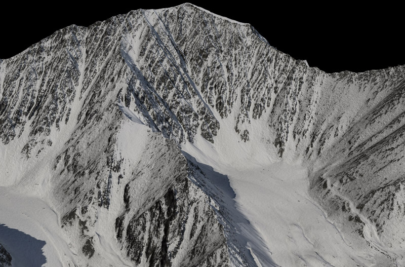
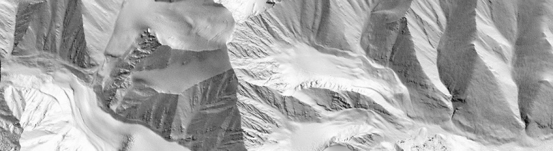
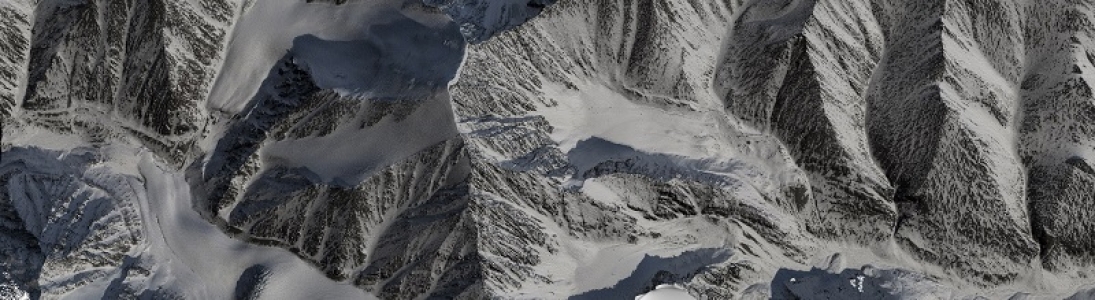
Because the data are digital, we can use visualization software to see it in 3D perspective. Here again is Mt Isto, with the orthoimage overlaid on terrain. Place your mouse over the image to see just the topography in shaded relief format. It is crucially important to understand that fodar creates both a DEM and a perfectly co-registered orthoimage at the same time. Other techniques such as lidar create only a DEM.
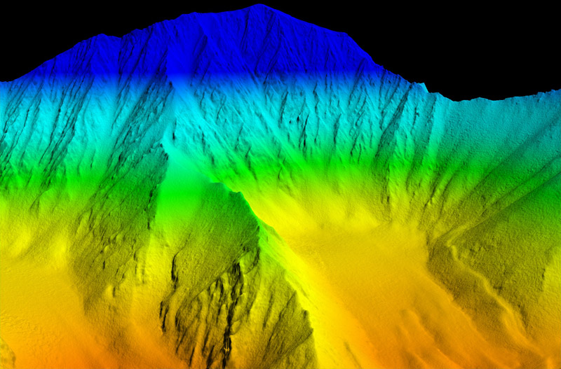
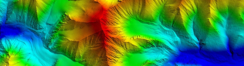
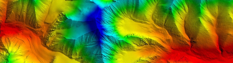
Here is the DEM again as a color slice. Mouse-over to see a different color scheme. Color schemes are arbitrary.
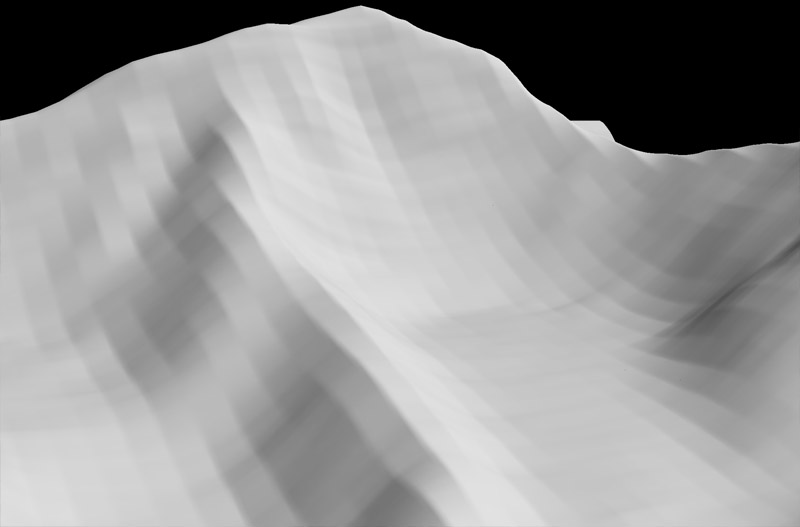
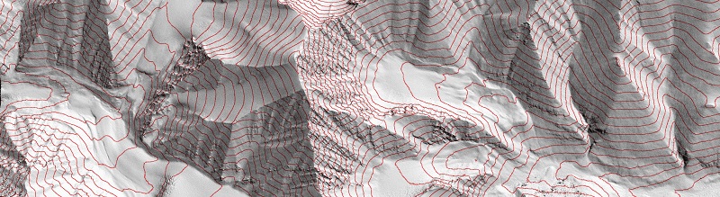
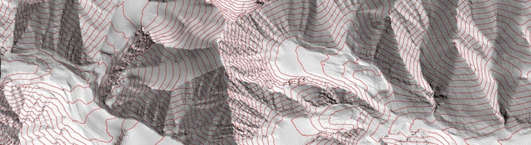
Here is the best DEM from the USGS of Mt Isto. Notice that you can see the individual pixels because the GSD is much coarser, about 50 m rather than the 50 cm Fodar DEM you will see when you mouse-over. Whether the increase is resolution is useful to you depends of course on your needs. In this case, not only can we resolve the individual glaciers in the Fodar DEM, but we can get a good sense of change over the 60 years between map acquisitions.
Accuracy, Precision and Noise Level
We have done extensive testing of the accuracy, precision and noise level of the fodar method of photogrammetry. Without using any ground control, our DEMs are always accurate in the realworld to within +/- 100 cm, and usually better than 30 cm, with the vertical offset typically being the largest. A single high-quality ground control point can reduce this accuracy to the precision level of the DEM. The precision of fodar, that is its repeatibility, is about +/- 10 cm. That is, if two fodar maps of the same area are made on the same day, subtracting those two maps should yield a map where all values are less than +/- 10 cm (assuming the realworld surface did not change). Depending on a variety of factors this precision can be reduced to +/- 5 cm and it can be as high as +/- 50 cm; the coarser the GSD, the lower the precision, and other factors contribute to precision levels. The precision errors take the form of small-scale warps and tilts within the DEM, largely due to slight misalignments between adjacent photos when creating the point cloud. The random noise level of fodar DEMs is about 1-3 cm. Because the noise level is much lower than the precision level, features as small as several centimeters in height can be resolved even though they are below the level of precision, but their absolute elevations are suspect at the 10 cm level.
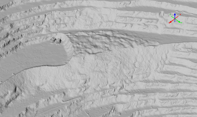
Here is a fodar shaded relief of an open-pit mine site. There is a shovel scooping up recently blasted rock and loading it into a dump truck to the left of center. After a week of work, the recently blasted rock is almost completely removed —mouse-over to see it. While flickering back and forth between the two images, pay particular attention to the ledges to the right and notice how little motion you see there. Only data precise to the 10 cm level can produce such perfect correspondence between DEMs, and most map-making methods are not nearly that precise.
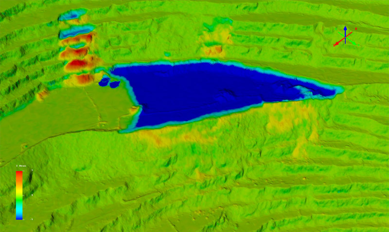
This is a difference image draped over topography. A difference image is created by subtracting (differencing) two DEMs, just as you might subtract two spreadsheets. A new DEM is created, where instead of each spreadsheet cell representing elevation it represents change in elevation. This difference DEM can then be colored like any DEM, where the colors themselves are arbitrary. In this case, green means no change, red means the surface was raised and blue means the surface was lowered. Note how this difference image clearly shows the rock that was removed by the trucks, but also shows several small detachments above and spillage from loading below it. The detachments show loss at their top (blue or dark green) and gain below (yellows and reds). On the lower levels, individual rocks can be seen in yellow; some of these rocks are the size of a basketball.
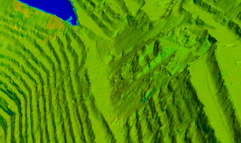
Here is another difference image of the same site, you can see the excavation of the previous images in the upper left. Green represents no change, and no change is apparent here until you look closer by mousing-over. The mouse-over shows two things. First is that the color scheme of a difference image is arbitrary — this image has the same data, but with colors stretched differently. The first image has blues to reds stretch to +/- 5 m, but the mouse-over image has the same colors stretched to +/- 30 cm, so each change in color represent a much smaller change in topography. At this color resolution, a fault line is revealed to be moving. A few weeks later, this fault released, causing a major landslide here. You can see the results of this landslide in the Applications section.
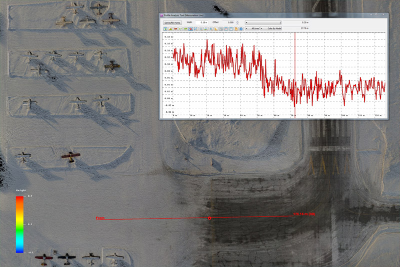
Here is the Fairbanks International Airport in winter. The runway is plowed down to tarmac but the taxi ways are packed so that ski planes can get around. The inset plot shows fodar snow depth, measured by subtracting a snow-free DEM from this one. The plot has 2 cm vertical ticks, showing a transition from 0 to 10 cm. The random noise (the jitter in the line) is about +/- 2 cm, yet a fairly smooth transition can be seen from 0 to 10 cm, indicating that we are measuring snow depth at the centimeter scale. Mouse-over to see the difference image. Here you will see how the plow trucks try to avoid the parked planes, leaving the snow thicker there.
There are several other types of noise in fodar DEMs. Photogrammetry works by matching features between photographs. For this to occur accurately, those features must exist and must not be moving. Features in this case are defined by contrast between adjacent pixels, like the edge of a rock or building. If there is no contrast in the photos, there are no features to match, and therefore no point cloud can be resolved there. Thus freshly fallen snow in deep shadows have much fewer features to match than windblown snow in the sun. It is rare that no contrast can be found, but those features may be at a larger spatial scale than the mission intended, so that rather than producing a 10 cm DEM it may only be possible to create a 40 cm DEM there. In the absence of contrast at the intended spatial scale, camera sensor noise can be misinterpreted by the software as contrast defining real features and be used in reconstructing topography, which will lead to increased noise since they are not real features. This occurs rarely, but when it does it is typically on the order of random pits and spikes of 1-5 meter amplitude about the true elevation and is something that can be filtered out through post-processing. Fodar also does not work well over liquid water bodies, as in calm conditions there is no contrast and under windy conditions the waves are moving. When the bed of the water body can be seen in the image, the contrast there will be used to reconstruct topography but the resulting elevations will not be as accurate as on land because the bending of light rays within the water has not been accounted for. Thus a shallow lake surface will appear to have an elevation, but it should be used with caution. If clouds and fog obscure the ground, their tops may be used to create elevation data, so the orthoimage must be examined to determined what is ground and what is cloud top. Because Fodar is a photographic process, part of the Fodar technique is to consider the optimal weather conditions for acquiring the raw data used in processing.
There is no minimum or maximum size of a fodar project. Typical sizes range from 20 to 200 square kilometers, but we have many projects over 3000 square kilometers. The constraints are typically more about weather (bigger projects take longer), fuel (is enough available where you need it), and budget. Another important consideration regarding areal coverage is the file size that results — a 10 km by 10 km area at 10 cm GSD will create 70 gigabytes worth of final DEM and orthoimage, not including the raw imagery. Most computers today have a difficult time handling such files. That’s why we developed FodarEarth, so these data can be shared online to almost any Windows computer.
Differences between lidar and fodar
Compared to lidar, fodar maps are just as precise, plus fodar produces a perfectly co-registered orthophoto whereas lidar only produces a DEM. The importance of an associated orthoimage should not be underestimated when trying to interpret small, subtle changes to the earth’s surface, as the images below demonstrate. Another issue with lidar is that there are many lidar manufacturers, many lidar models, and many lidar operators, and thus there is a wide variety in lidar quality both in terms of what is being offered and what gets delivered, and this can be troublesome for end-users. While the same could be said of SfM-based photogrammetry, our goal in giving fodar its own name is to distinguish from SfM techniques of lower accuracy. Perhaps most importantly, fodar is much less expensive than lidar, allowing end-users to not only make one good map of their site, but a time-series of them. With this time series, the accuracy and precision of the maps can be directly measured. From our view, it should be a requirement of every project that the area of interest be acquired twice – either the same day or as part of a time-series – to eliminate all guess work in terms of accuracy and precision. The ability to affordably make time-series of elevation change of entire watersheds on the centimeter-scale also has the potential to revolutionize earth sciences.
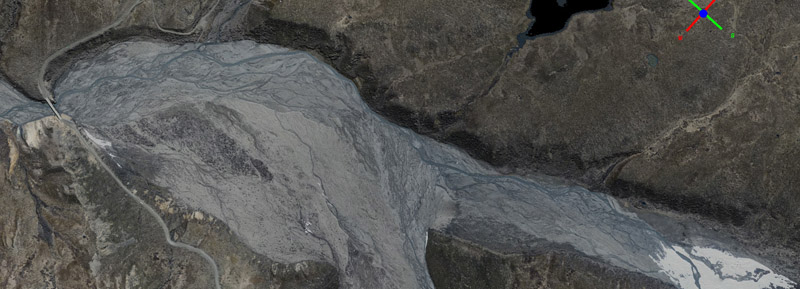
Here is a section of the Toklat River in Denali National Park in June. Mouse-over to see it in August. You can see from the images that the stream channels have changed considerably.
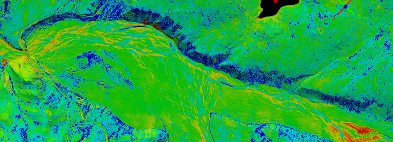
Here is the difference image between June and August. Light green means no change, yellows and reds mean the surface was higher in June and blue mean it was lower. There is a lot of both real change and water-related noise. Because the streams were shallow or dirty, both DEMs reconstructed topography that is not accurate. When differenced, this appears to show a change in elevation. While the change in elevation is real, the elevations have errors, probably on the order of tens of centimeters. Without a perfectly co-registered image that was simultaneously acquired (mouse-over to see one), it would be difficult if not impossible to distinguish changes in water level from changes in the surrounding gravel bars. Similarly, without the image, it would be difficult to distinguish snow and ice melt from gravel bar change.